An improved Adam Algorithm using look-ahead An Zhu
Yu Meng
Changjiang Zhang
Dept. of Computer Science Wenzhou-Kean University 88 Daxue road Wenzhou, China (+86)18858716728
Dept. of Biological Science Wenzhou-Kean University 88 Daxue road Wenzhou, China (+86)577-5587-0775
Dept. of Computer Science Wenzhou-Kean University 88 Daxue road Wenzhou, China (+86)577-5587-0736
[email protected]
[email protected]
[email protected]
ABSTRACT Adam is a state-of-art algorithm to optimize stochastic objective function. In this paper we proposed the Adam with Look-ahead (AWL), an updated version by applying look-ahead method with a hyperparameter. We firstly performed convergence analysis, showing that AWL has similar convergence properties as Adam. Then we conducted experiments to compare AWL with Adam on two models of logistic regression and two layers fully connected neural network. Results demonstrated that AWL outperforms the Adam with higher accuracy and less convergence time. Therefore, our newly proposed algorithm AWL may have great potential to be widely utilized in many fields of science and engineering. CCS Concepts • Computing methodologies➝Artificial intelligence➝ Machine learning➝Machine learning algorithms. Keywords Machine learning; Gradient-based Optimizer; Adam; Look-ahead 1. INTRODUCTION The Stochastic gradient-based optimization methods, such as stochastic gradient decent (SGD) and batch gradient decent (BGD), are widely used in machine learning, deep learning, artificial intelligence and other related areas [1]. The optimal parameters can be determined using stochastic gradient-based optimization methods when training the machine learning model. Thus, the cost function, which represents how accurate our predicted values are and is differentiable with w.r.t as its parameters, can obtain the minimum value. Gradient decent is theoretically efficient as compared to other methods, considering that it only requires the first order derivate of the parameters to update. In turn, higher-order methods are limited to be compatible with high-dimensional parameters spaces which are crucial in deep learning Unlike BGD which requires a batch of training data as input, SGD only takes single training data and has been shown to be portable in deep learning problem [2]. Adam[3], an update to RMSProp [4] by integrating Momentum [5], is the state-of-art first-order gradient based optimizer having superior computational efficiency with little memory requirements. SAMPLE: Permission to make digital or hard copies of all or part of this work for personal or classroom use is granted without fee provided that copies are not made or distributed for profit or commercial advantage and that copies bear this notice and the full citation on the first page. To copy otherwise, or republish, to post on servers or to redistribute to lists, requires prior specific permission and/or a fee. Conference’10, Month 1–2, 2010, City, State, Country. Copyright 2010 ACM 1-58113-000-0/00/0010 …$15.00. DOI: http://dx.doi.org/10.1145/12345.67890
It has been reported that Momentum can be improved by applying look-ahead. Nesterov Momentum, the updated version was shown to have higher accuracy as compared with the original one [5]. Here, we propose the Adam with Look-ahead (AWL), an improved update to Adam that requires first-order gradients with a little more memory space. AWL will use the moments to perform the lookahead, and the look-ahead parameters will be applied to get the gradients. Then, the first and second moments will be updated based on the new gradients. Furthermore, the new moments will be used to update the parameters. Finally, in order to implement AWL more efficiently, we will use a mathematically equivalent formula to avoid those look-ahead parameters and introduce a new hyper parameter to control the strength of look ahead. In section 2 we described the design of AWL integrating the discussion about the Momentum, Adam, RMSprop, Nesterov Momentum and their relevance to AWL. In section 3 we detailed the updates in AWL algorithm, and provided two version of AWL. In section 4 we performed a convergence analysis of AWL. Finally, in section 5 experiments were conducted and results demonstrated that AWL outperforms Adam with less time to converge on two models. AWL might display better convergence when the learning rate is large and not optimal. 2. DESIGN Inspired by the fact that Nesterov Momentum was improved by applying look-ahead on Momentum [5], we aim to update Adam in the same manner. Additionally, we also introduced a new hyper parameter to control the strength of look-ahead. Adam is a first-order gradient-based optimizer, which was proposed by Diederik and Jimmy in 2015[1]. As a combination of two outstanding update methods, Momentum, which use first order moment to do the update, and Ada-Grad [6] or RMSprop[4], which use the second order moment to do the update, it has outperformed a variety of optimizers and become popular in solving deep learning problems. The core part of Adam algorithm is as follows [1]: m = 𝛽1 ∙ m + (1 − 𝛽1 ) ∙ 𝑑𝑥 v = 𝛽2 ∙ v + (1 − 𝛽2 ) ∙ 𝑑𝑥2 x −= α ∙
m √v+𝜖
𝛽1 and 𝛽2 are two constants, and x represents for the
parameters to be updated and dx is derivative vector of x. Notice here m is used to store the first order moment similar to what Momentum update did, and v is used to store the second order moment similar to what RMSprop update did. Then it makes updates based on both of the moments. To develop AWL, we modified the look-ahead technique to be
more compatible with Adam. One great example of look-ahead is Nesterov Momentum. Compared with Momentum, Nesterov Momentum obtains more promising converge property theoretically, and consistently works better than standard Momentum in practice. The core idea behind look-ahead is that parts of moments are added to the update despite the current gradient, which suggests there are certain points we know the parameters will go through before we calculate the gradient. Therefore, it makes sense to calculate the gradient at that point instead of the point the parameters really are. Figure1 shows the comparison between standard Momentum and Nesterov Momentum.
While 𝑥𝑡 not converged do t← 𝑡+1 𝑥𝑝 ← 𝑥𝑡−1 − α ∙ 0.9 ∙
𝑚𝑡−1 √𝑣𝑡−1 +𝜖
(Update
look
ahead
parameter ) 𝑔𝑡 ← ∇𝑥 𝑓𝑡 (𝑥𝑝 ) (obtain the gradient of the look ahead parameter) 𝑚𝑡 ← 𝛽1 ∙ 𝑚𝑡−1 + (1 − 𝛽1 ) ∙ 𝑔𝑡 (update first moment estimate ) 𝑣𝑡 ← 𝛽2 ∙ 𝑣𝑡−1 + (1 − 𝛽2 ) ∙ 𝑔𝑡2 moment estimate) 𝑥𝑡 ← 𝑥𝑡−1 − α ∙
𝑚𝑡 √𝑣𝑡 +𝜖
(update
second
(update parameter)
end while Return 𝑥𝑡 (Resulting parameters) In AWL, an approximation position of the updated point will be estimated by implementing look-ahead and the point’s gradient will be utilized instead. Appling look-ahead technique is shown to improve Momentum by a little [5]. In stage 2, we further improve the Algorithm by removing the look-ahead parameter 𝑥𝑝 to save the memory space while introducing a new hyper-parameter γ to control the strength of look-ahead. This hyperparameter would not affect the convergence of AWL (Section 3):
Figure 1. Comparison between Momentum and Nesterov Momentum on one step of update. Notice the only difference is that gradient in step a is calculated by the parameters points gradient. However, gradient in step b is calculated by the estimated point’s gradient.
3. ALGORITHM We developed AWL in two stages. In stage 1, we add look ahead technique into Adam. Notice that the original Adam Algorithm contains a few lines for bias correction, based on the fact that m and v are initialized and therefore biased at 0. We do not include those terms for more clear expression. Stage 1: This is an intermediate version. This version is not for implementing but a necessary part to understand how we generate AWL from Adam. We also discussed another version of AWL without look-ahead parameters in this section. 𝑔𝑡2 is the element wise square of 𝑔𝑡 . For machine learning problemsα = 10−3 , 𝛽1 = 0.9, 𝛽2 = 0.999 𝑎𝑛𝑑 𝜖 = 10−8 . In some cases α is treated as a hyper-parameter. Require: α learning rate Require: 𝛽1 , 𝛽2 within 0 to 1, Exponential decay rates for moment estimates Require: 𝑓(𝑥): cost function Require: 𝑥0 : initial parameter vector 𝑥𝑝 ← 0 (initialize look ahead parameter) 𝑚0 ← 0 ( initialize first order moment vector) 𝑣0 ← 0 ( initialize second order moment vector) 𝑡 ← 0 ( initialize timestep)
Stage2: Final version of AWL, without look-ahead parameters. This is the final AWL algorithm, which is used for convergence analysis and implementation.𝑔𝑡2 is the element wise square of 𝑔𝑡 . ℎ𝑖 𝑖𝑠 𝑎𝑛 intermediate variable, which contains the calculation results of two moments. γ is the new hyperparameter we introduced to control the strength of look ahead. Notice that when γ = 0.9 Stage 2 algorithm is identical with stage 1 algorithm. For machine learning problems α = 10−3 , 𝛽1 = 0.9, 𝛽2 = 0.999 𝑎𝑛𝑑 𝜖 = 10−8 . In some cases α is also treated as a hyperparameter. Require: α learning rate Require: 𝛽1 , 𝛽2 within 0 to 1, Exponential decay rates for moment estimates Require: 𝑓(𝑥): cost function Require: 𝑥0 : initial parameter vector 𝑚0 ← 0 ( initialize first order moment vector) 𝑣0 ← 0 ( initialize second order moment vector) 𝑡 ← 0 ( initialize timestep) ℎ0 ← 0 ( initialize intermidiate variable) While 𝑥𝑡 not converged do 𝑡 ← 𝑡+1 𝑔𝑡 ← ∇𝑥 𝑓𝑡 (𝑥𝑡−1 ) (obtain the gradient of the look ahead parameter) 𝑚𝑡 ← 𝛽1 ∙ 𝑚𝑡−1 + (1 − 𝛽1 ) ∙ 𝑔𝑡 (update first moment estimate ) 𝑣𝑡 ← 𝛽2 ∙ 𝑣𝑡−1 + (1 − 𝛽2 ) ∙ 𝑔𝑡2 moment estimate)
(update
second
ℎ𝑡 ←
𝑚𝑡 √𝑣𝑡 +𝜖
𝑥𝑡 ← 𝑥𝑡−1 − α ∙ ((1 + γ ) ∙ ℎ𝑡 − γ ∙ ℎ𝑡−1 ) (update parameter) end while Return 𝑥𝑡 (Resulting parameters)
4. CONVERGENCE ANALYSIS Suppose the learning rate does not change overtime, every time of applying the final AWL algorithm will add negative α ∙ ((1 + γ ) ∙ ℎ𝑡 − γ ∙ ℎ𝑡−1 ) to parameters, which add up to∑𝑛𝑡=0 𝛼 ∙ ((1 + 𝛾 ) ∙ ℎ𝑡 − 𝛾 ∙ ℎ𝑡−1 ) . This formula equals to α ∙ (γ ∙ ℎ𝑛 − γ ∙ ℎ0 ) + ∑𝑛𝑡=0 𝛼 ∙ ℎ𝑡 , where the ∑𝑛𝑡=0 𝛼 ∙ ℎ𝑡 is exactly as Adam update. ℎ0 = 0, 𝛼 𝑎𝑛𝑑 𝛾 are constant. Besides, ℎ𝑛 is usually close to zero when SGD performs correctly, since it is calculated by the last moment vectors, so α ∙ (γ ∙ ℎ𝑛 − γ ∙ ℎ0 ) = α ∙ γ ∙ ℎ𝑛 ≈ 0. Therefore, AWL should have similar convergence as Adam. Notice 𝛼 is our newly added hyperparameter, which would not affect AWL convergence if being set as a constant.
is slightly lower than the minimum of Adam and faster (50 epoch for AWL vs. 67 epoch for Adam) (Figure 2). It suggested that AWL can use first and second order Momentum more efficiently, and provide more accurate estimates on gradient. AWL also shows more outstanding properties compared with Adam. We applied a grid search on hyper-parameters to find the optimized hyper-parameter. As shown in Figure 3. As the learning rate decreases, AWL and Adam demonstrated similar validation cost values, suggesting that they both have similar properties of convergence. However, when the learning rate is higher, AWL displayed a better performance than Adam. Results indicated that AWL may use higher learning rate to achieve faster training, while maintaining acceptable accuracy.
5. EXPERIMENTS To evaluate the improved method, we compared the performance of AWL with the original Adam on different popular machine models including logistic regression and a two layers fully connected neural networks with the large dataset in wide usage. The parameters were initialized to be the same and the hyper parameter like learning rate and regulation are set to be the most optimal.
5.1 Experiment: Logistic Regression Logistic regression is suitable for comparing optimal method without worrying about local minimum. AWL and Adam were compared on multi-class logistic regression model with L2regularization using the MNIST dataset on mini batch of 128. The 1 step size is adjusted by decay. According to Figure 2 we found √t
that AWL yields similar convergence as Adam with lower cost and less iterations to reach the optimal results.
Figure 2: Comparison between Adam and AWL on Logistic Regression. Logistic regression validation and test cost of negative log likelihood with optimal hyper parameters As discussed in section 3 AWL possesses the similar convergence as Adam. We examined the improvement by setting the maximum iterations over entire dataset to 100. The minimum value of AWL
Figure 3. Comparison between Adam and AWL on Logistic Regression during selecting hyperparameters. The two hyperparameters are learning rate and L2 regulation weight. Each point represents a combination of learning rate and L2 regulation. The model was trained for 40 epoch for each combination. Notice that the learning rate decreases rapidly from 0.3 to 0.0003 over the whole x-axis.
5.2 Experiment: Multi-Layer Neural Networks Multi-layer neural networks are widely used in machine learning, for its strength on dealing with high dimensional input space. Although, multi-layer neural networks are normally used on nonconvex objective function, Adam has still been considered superior to other methods. We implemented model that is consistent with the one Adam was analyzed on; a neural model with two fully connected hidden layers with 1000 hidden units each. ReLU activation is used with minibatch size of 128. Multi-layer neural network is famous for it can easily go overfitted, dropout [7] is one of the modern technique to address overfitting problem. We compared AWL with Adam on a multilayer neural network, which was originally implemented by Poole [8]. Figure 4 suggested that AWL possesses similar convergence as Adam with lower cost, which is consistent with results from Logistic regression (Figure 2).
8. REFERENCES [1] Kingma, D. and Ba, J. 2014. Adam: A Method for Stochastic Optimization. arXiv preprint arXiv:1412.6980 [2] Bottou, L. 2010. Large-scale machine learning with stochastic gradient descent. In Proceedings of COMPSTAT'2010, 177-186. [3] Ngiam, J., Coates, A., Lahiri, A., Prochnow, B., Le, Q. V., and Ng, A. Y. 2011. On optimization methods for deep learning. In Proceedings of the 28th International Conference on Machine Learning (ICML-11) .265-272. [4] Nesterov, Y. 1983. A method for unconstrained convex minimization problem with the rate of convergence O (1/k2). In Doklady an SSSR, 543-547. Figure 4. Training of a two layers fully connect neural network on MNIST images. Using batch stochastic gradient decent with dropout.
6. CONCLUSIONS We introduced and implemented AWL, which is an improved version of Adam by applying look-ahead and a hyperparameter. Look-ahead allows the algorithm to achieve better estimated gradients and to process more efficiently. The hyperparameter helps control look-ahead better. Convergence analysis suggested AWL will display similar convergence as Adam in convex problems. Experimental results demonstrated that AWL has higher accuracy and efficiency as compared to Adam in both convex and non-convex problems. To sum up, AWL outperforms Adam, and AWL may have better utilization in many fields of science and engineering.
7. ACKNOWLEDGMENTS This work is supported by the Student-Partnering-Faculty research project(WKU201617003) and Zhejiang province natural science foundation grant(LY16H080008) .
[5] Duchi, J., Hazan, E., and Singer, Y. 2011. Adaptive subgradient methods for online learning and stochastic optimization. Journal of Machine Learning Research, 12(Jul), 2121-2159. [6] Tieleman, T., Hinton, G. 2012. Lecture 6.5-rmsprop: Divide the gradient by a running average of its recent magnitude. COURSERA: Neural Networks for Machine Learning, 4(2). [7] Srivastava, N., Hinton, G. E., Krizhevsky, A., Sutskever, I., and Salakhutdinov, R. 2014. Dropout: a simple way to prevent neural networks from overfitting. Journal of Machine Learning Research, 15(1), 1929-1958. [8] Sohl-Dickstein, J., Poole, B., and Ganguli, S. 2014 Fast large-scale optimization by unifying stochastic gradient and quasi-newton methods. In Proceedings of the 31st International Conference on Machine Learning (ICML-14), 604–612.