Hindawi Publishing Corporation Mathematical Problems in Engineering Volume 2014, Article ID 658915, 11 pages http://dx.doi.org/10.1155/2014/658915
Research Article An Improved Adaptive Deconvolution Algorithm for Single Image Deblurring Hsin-Che Tsai and Jiunn-Lin Wu Department of Computer Science and Engineering, National Chung Hsing University, Taichung 40227, Taiwan Correspondence should be addressed to Jiunn-Lin Wu;
[email protected] Received 3 October 2013; Accepted 3 January 2014; Published 19 February 2014 Academic Editor: Yi-Hung Liu Copyright © 2014 H.-C. Tsai and J.-L. Wu. This is an open access article distributed under the Creative Commons Attribution License, which permits unrestricted use, distribution, and reproduction in any medium, provided the original work is properly cited. One of the most common defects in digital photography is motion blur caused by camera shake. Shift-invariant motion blur can be modeled as a convolution of the true latent image and a point spread function (PSF) with additive noise. The goal of image deconvolution is to reconstruct a latent image from a degraded image. However, ringing is inevitable artifacts arising in the deconvolution stage. To suppress undesirable artifacts, regularization based methods have been proposed using natural image priors to overcome the ill-posedness of deconvolution problem. When the estimated PSF is erroneous to some extent or the PSF size is large, conventional regularization to reduce ringing would lead to loss of image details. This paper focuses on the nonblind deconvolution by adaptive regularization which preserves image details, while suppressing ringing artifacts. The way is to control the regularization weight adaptively according to the image local characteristics. We adopt elaborated reference maps that indicate the edge strength so that textured and smooth regions can be distinguished. Then we impose an appropriate constraint on the optimization process. The experiments’ results on both synthesized and real images show that our method can restore latent image with much fewer ringing and favors the sharp edges.
1. Introduction Image blurring is one of the prime causes of poor image quality in digital photography. The one main cause of blurry images is motion blur caused by camera shake. If a motion blur is linear shift invariant, the blurring process can be generally modeled as a convolution of the true latent image and a point spread function (PSF) with additive noise: 𝐵 = 𝐾 ⊗ 𝐼 + 𝑁,
(1)
where 𝐵 is the degraded image, 𝐼 is the true latent image, 𝐾 is the PSF or a motion blur kernel which describes the trace of a sensor, 𝑁 is the additive noise introduced during image acquisition, and ⊗ denotes the convolution operator. The goal of image deblurring is to reconstruct a latent image 𝐼 from degraded image 𝐵. To remove motion blur, we need to estimate the PSF and restore a latent image through deconvolution. Existing single image deblurring methods can be further categorized into two classes. If both the PSF and the latent image are
unknown, the challenging problem is called blind deconvolution. Although great progresses have been achieved in the recent years [1–4], blind case is severely ill-posed problem because the number of unknowns exceeds the number of observed data. In contrast to the former, if the PSF is assumed to be known or computed in other ways, the problem is reduced to estimating the latent image alone. This is called nonblind deconvolution. However, the nonblind case is still an ill-conditioned problem that has to do with the presence of image noise. Slight mismatches between the PSF used by the method and the true blurring PSF also lead to poor deblurring results. Unfortunately, the deconvolved result usually contains unpleasant artifacts even if the PSF is exactly known or well estimated. The main visually disturbing artifact is ringing that appears around strong edges. Because the PSF is often bandlimited with a sharp frequency cutoff, that will be zero or near-zero values in its frequency response. Thus the direct inverse of the PSF causes large amplification of signal and noise.
2
Mathematical Problems in Engineering
Since the estimated PSF is usually inaccurate and the real blurred image is also noisy, many underconstrained factors will affect the amplification of ringing. To reduce undesirable artifacts, various regularization techniques have been proposed using image priors to improve nonblind deconvolution methods [5–10]. The most commonly used priors are those which encourage the image gradients to a set of derivative filters to follow heavy-tailed distribution. However, strong regularization to reduce severe artifacts destroys the image details in the deconvolved result. Weak regularization preserves image details well, but it does not remove artifacts tellingly. The challenge of this work is how to balance the details recovery and ringing suppression. In this paper, we focus on non-blind deconvolution with adaptive regularization that controls the regularization strength according to the image local characteristics. This strategy reduces ringing artifacts in a smooth region effectively and preserves image details in a textured region simultaneously. First, we estimate the reference maps in the scale space. At the coarsest scale, we are able to extract reasonably main strong edges. Comparing the texture information of multiscale results, we can make the elaborated reference map that differentiates the edge property of textured region and smooth region. Second, regularization strength is controlled adaptively referring to these maps. Then, we apply appropriate regularization with hyper-Laplacian prior to image deconvolution so that the sharp edges can be eventually recovered. To solve the optimization process, we adopt Krishnan’s [7] fast algorithm. It is performed fast in the frequency domain using fast Fourier transforms (FFTs). The experimental results show that our nonblind deconvolution can produce latent image with much fewer ringing and preserve the sharp edges.
2. Regularization Formulation Assuming that the PSF is known or computed in other ways, our method focuses on recovering the sharp image from the blurred image. To reduce undesirable artifacts, most advanced regularization techniques are proposed using the prior of nature image in the gradient domain. We now introduce the regularization formulation. From a probabilistic perspective, we seek maximum a posteriori (MAP) estimate of latent image 𝐼 in Bayesian framework: 𝑝 (𝐼 | 𝐵) ∝ 𝑝 (𝐵 | 𝐼) 𝑝 (𝐼) ,
(2)
where 𝑝(𝐵 | 𝐼) represents the likelihood and 𝑝(𝐼) denotes the priors on the latent image. Maximizing 𝑝(𝐼 | 𝐵) is equivalent to minimizing the cost − log 𝑝(𝐼 | 𝐵): − log 𝑝 (𝐼 | 𝐵) = − log 𝑝 (𝐵 | 𝐼) − log 𝑝 (𝐼) .
(3)
The MAP solution of 𝐼 can be obtained by minimizing the cost function above. We now define these two terms. The likelihood of a degraded image given the latent image is based on the common blur model 𝑁 = 𝐵 − 𝐾 ⊗ 𝐼. Assuming that the noise is modeled as a set of independent and identically distributed (i.i.d.) noise random variables for all pixels, each
of which follows a Gaussian distribution, we can express the likelihood with Gaussian variance 𝜎2 as 2
2
𝑝 (𝐵 | 𝐼) ∝ 𝑒−(1/2𝜎 )‖𝐵−𝐾⊗𝐼‖ .
(4)
Furthermore, recent research in natural image statistics shows that image gradients follow a heavy-tailed distribution. These distributions are well modeled by a hyper-Laplacian prior and have proven effective priors for deblurring problem. In this paper, we utilize the hyper-Laplacian prior to regularize the solution and it can be modeled as 2
𝑝 (𝐼) ∝ 𝑒−𝛼 ∑𝑘=1 |𝑓𝑘 ⊗𝐼|
𝑞
with 0.5 ≤ 𝑞 ≤ 0.8,
(5)
where 𝑞 is a positive exponent value set in the range of 0.5 ≤ 𝑞 ≤ 0.8 as suggested by Krishnan and Fargus [7]. In this work, we unify the use of 2/3 for 𝑞 value. The 𝑓𝑘 denotes the simple horizontal and vertical first-order derivative filters. It can also be useful to include second-order derivative filters or the more sophisticated filters. With the Gaussian noise likelihood and the hyper-Laplacian image prior, (3) can be represented by the following minimization problem: 𝑛
2
𝑖=1
𝑘=1
𝑞 arg min ∑ ((𝐵 − 𝐾 ⊗ 𝐼)2𝑖 + 𝜂 ∑ (𝑓𝑘 ⊗ 𝐼)𝑖 ) , 𝐼
(6)
where 𝑖 is an index running through all pixels, 𝑛 is the whole pixels in the image, and weighting coefficient 𝜂 = 2𝛼𝜎2 controls the strength of the regularization term. For simplicity, 𝑓1 = [1 − 1] and 𝑓2 = [1 − 1]𝑇 are two firstorder derivative filters. We search for the 𝐼 which minimizes the reconstruction error ‖𝐵 − 𝐾 ⊗ 𝐼‖2 , with the image prior preferring 𝐼 to favor the correct sharp explanation. However, to analyze the formulation of Equation (6), the above conventional regularization’s weighting coefficient 𝜂 is applied to all pixels with the same strength. When the estimated PSF is inaccurate or the PSF size is large, it usually adds strong regularization weight for suppressing ringing around the edges. But it also destroys the image details in the deconvolved result, and this is inevitable problem since perfect PSF estimation is impossible. In addition, the weak regularization weight preserves major details well, but it does not remove artifacts effectively.
3. The Proposed Method To balance the details recovery and ringing suppression, the main ideal of our approach is to control the regularization weight adaptively according to the image local characteristics. This means that we need strong regularization for the smooth regions and weak regularization for the sharp edges. Our estimated maps further consider the edge property of image textured regions. In this chapter, we will explain each step of our algorithm in detail. That includes how to estimate reference map and perform the adaptive regularization in the deconvolution stage. Finally, we supply some added improvement to obtain better results. Figure 1 shows the overall process of our nonblind deconvolution method.
Mathematical Problems in Engineering
3
t= t+1 PSF K
Blurred image B Map estimation t=0 Reference map Mref
No
+ Adaptive deconvolution
Deconvolved image I
Stop iteration? Yes Deblurred image
Figure 1: Overview of our adaptive deconvolution framework.
3.1. Reference Map Estimation. Inspired by the local constraint idea [8, 9, 11], the reference map is designed for classifying the smooth regions and different edge regions correctly. Reference map is used for deconvolution with adaptive regularization and can apply the right image characteristics information to control the local weight of deblurring. In fact, the classified texture regions also contain the main strong edges and some smaller or fainter edges. Compared to the smaller or fainter edges, the extracted main edges are the important visible regions, and those need more weak regularization to preserve the sharp features. In addition, we should add strong regularization for the classified smooth regions to reduce the most noticeable artifacts since the ringing artifacts are usually propagated in the smooth areas. Based on these observations, we estimate the reference maps in the multiscale space. We first build a pyramid 𝐿
{𝐵𝑙 }𝑙=0 of the full resolution input blurred image 𝐵 using bilinear downsampling. Our goal is to combine different edge information from coarse to fine layers. So we perform the map estimation approach in each scale and distinguish its different regions. At the coarsest scale, we are able to extract reasonably main strong edges of the image. In the next finer scale, we gradually extract more and more small edge details. Finally, all estimated maps from different scale results combine to form one elaborated reference map. The estimation is guided to a good map by concentrating on the main edges of the input image and progressively dealing with smaller and smoother details. But it is difficult to obtain
correct edge information from the blurred image directly, so the map is renewed from every deconvolved result during each iteration time. We now describe how to produce and combine the estimated reference maps. The initial reference map is estimated from the input blurred image. Since the locally smooth region which has no edges information is still smooth after blurring, the edge areas of blurred image will be affected. Inspired by this idea, we compute the edge strength and use predefined threshold to classify different regions. The edge strength at located pixel 𝑖 is defined as follows: Eg (𝑖) =
(∑ℎ∈𝑊𝑥 ℎ + ∑V∈𝑊𝑦 V) 𝑁total
,
(7)
where Eg(𝑖) denotes the edge strength response at pixel 𝑖 on the observed image. 𝑊 is the 3 × 3 window whose center is located on 𝑖, 𝑊𝑥 = 𝑊 ⊗ [1 − 1], 𝑊𝑦 = 𝑊 ⊗ [1 − 1]𝑇 , and 𝑁total is the total number of pixels in default window. If the computed edge strength value is smaller than a predefined threshold 𝑇, which is set to 3 × 10⁻² in our experiment, we will regard the center pixel 𝑖 as in smooth region Ω, that is, 𝑖 ∈ Ω: 1 if Eg (𝑖) < 𝑇 𝑀𝑖𝑙 = { 0 otherwise.
(8)
Since the texture regions which is classified by (7) also contain the main strong edges and some smaller edges, we aim to further improve the estimated results. The improved extracting method includes the following steps. Firstly, we 𝐿
build a pyramid {𝐵𝑙 }𝑙=0 of the blurred image. At each scale 𝑙, the edge strength Eg(𝑖) is computed in every level and then is upsampled. It means that this step will produce 𝑙 number binary maps. Finally, we sum all the edge intensities at the same pixel location and run through all pixels. Now we get a new reference map after normalization process, which is shown in Figure 2(b), and the smooth region Ω is shown as the set of all white pixels. The strongest edges are indicated by the most dark pixels and the other gray level pixels mean the smaller or fainter edges. Hence, we define this extracting step using the multiscale approach of the observed image as: 𝑀ref =
∑𝐿𝑙=0 𝑀𝑙 , 𝐿
(9)
where 𝑀𝑙 is the binary map at the 𝑙th level of the images pyramid by (8), and 𝐿 denotes the total scale layers, for example, 𝐿 is set to 3 levers in our implementation. In (9), the final map 𝑀ref is extracted by summing up all the intensity values of those upsampling maps and normalizing the results. We gradually recover more and more image details by an iterative deconvolution algorithm because it can refine the result until convergence. Obviously, the deconvolved image with initial adaptive regularization shows much better edge information than does the input blurred image. Thus, at the following reference map estimation, we use the deconvolved
4
Mathematical Problems in Engineering
(a)
(b)
(c)
(d)
Figure 2: Reference map estimation. (a) Input blurred image. (b) First reference map is estimated from the blurred image. It can locally compute smooth regions and distinguish different edge regions. (c) The deconvolved image with the first adaptive regularization. (d) Second reference map is estimated from previous deconvolved result.
result from the previous iteration to distinguish different edge regions elaborately. We also adopt the same criterion to extract map. Second estimated result is represented in Figure 2(d). The map will be renewed from the earlier deconvolved result after each iteration. 3.2. Image Deconvolution with Adaptive Regularization. Now, we would like to seek the MAP solution for the latent image in the deconvolution stage. But the limitation of conventional regularization is that the same value of weighting coefficient 𝜂 is applied to whole pixels. To overcome this fault and balance the image quality, our method introduces an improvement, that is, to apply appropriate regularization weight according to the local characteristics. So, the adaptive regularization is performed based on the estimated reference map during each iteration time. Based on this idea, we simply modify (6) as follows: 𝑛
2
𝑖=1
𝑘=1
𝑞 arg min ∑ ((𝐵 − 𝐾 ⊗ 𝐼)2𝑖 + 𝜂𝑝 ∑ (𝑓𝑘 ⊗ 𝐼)𝑖 ) , 𝐼
(10)
where the weighting coefficient 𝜂𝑝 is adjusted based on the estimated reference map. It provides a basis to adaptively suppress the ringing effects in different regions. The effect of adaptive regularization in deconvolution result is represented in Figure 3. In comparison, our result exhibits sharper image detail and fewer artifacts. However, the use of sparse distributions with 𝑞 < 1 makes the optimization problem nonconvex. It becomes slow
to solve the approximation. Using the half-quadratic splitting, Krishnan’s [7] fast algorithm introduces two auxiliary variables 𝜔1 and 𝜔2 at each pixel to move the (𝑓𝑘 ⊗ 𝐼)𝑖 terms outside the | ⋅ |𝑞 expression. Thus, (10) can be converted to the following optimization problem: 𝑛
arg min∑ ((𝐵 − 𝐾 ⊗ 𝐼)2𝑖 𝐼,𝜔
𝑖=1
+
𝛽 2 2 ((𝑓1 ⊗ 𝐼 − 𝜔1 )𝑖 + (𝑓2 ⊗ 𝐼 − 𝜔2 )𝑖 ) 2
(11)
𝑞 𝑞 + 𝜂𝑃 ((𝜔1 )𝑖 + (𝜔2 )𝑖 )) , where (𝑓𝑘 ⊗ 𝐼 − 𝜔𝑘 )2 term is for constraint of 𝑓𝑘 ⊗ 𝐼 = 𝜔𝑘 and 𝛽 is a control parameter that we will vary during the iteration process. As 𝛽 parameter becomes large, the solution of (13) converges into that of (12). This scheme is also called alternating minimization [12] where we adopt a common technique for image restoration. Minimizing (13) for a fixed 𝛽 can be performed by alternating two steps. This means that we solve 𝜔 and 𝐼, respectively. One subproblem is to solve 𝜔1 and 𝜔2 , which is called 𝜔 subproblem. First, the initial 𝐼 is set to the input blurred image 𝐵. Given a fixed 𝐼, finding the optimal 𝜔 can be simplified into the following optimization problem: ( arg min 𝜔
𝜆𝑃 𝑞 𝛽 |𝜔| + (𝜔 − ])2 ) , 2 2
(12)
Mathematical Problems in Engineering
5
(a)
(b)
(c)
Figure 3: Effect of deconvolution with adaptive regularization. (a) The deconvolved result by Krishnan’s [7] algorithm with the same weighting value. (b) Our deconvolved result with different 𝜂𝑝 weighting values according to the local characteristics as defined above. (c) Close-ups of two image regions for comparison.
where the value ] = (𝑓𝑘 ⊗ 𝐼). For convenient calculation, 𝜂𝑝 is replaced with 𝜆 𝑝 /2, and it does not affect the performance. Inparticular for the case 𝑞 = 2/3, the 𝜔 satisfying the above equation is the analytical solution of the following quartic polynomial: 𝜔4 − 3]𝜔3 + 3]2 𝜔2 − ]3 𝜔 +
𝜆3𝑝 27𝛽3
= 0;
following optimization problem. Equation (11) is modified as arg min ((𝐵 − 𝐾 ⊗ 𝐼)2 𝐼
𝛽 2 2 + ((𝑓1 ⊗ 𝐼 − 𝜔1 ) + (𝑓2 ⊗ 𝐼 − 𝜔2 ) )) ; 2
the 𝐼 subproblem can be optimized by setting the derivative of the cost function to zero. So, (14) is quadratic in 𝐼. The optimal 𝐼 is 2 2 (𝐹1𝑇 𝐹1 + 𝐹2𝑇 𝐹2 + 𝐾𝑇𝐾) 𝐼 = 𝐹1𝑇 𝜔1 + 𝐹2𝑇 𝜔2 + 𝐾𝑇 𝐵; (15) 𝛽 𝛽
(13)
to find and select the correct roots of the above quartic polynomial, we adopt Krishnan’s approach, as detailed in [7]. They numerically solve (12) for all pixels using a lookup table to find 𝜔. Second, we briefly describe the 𝐼 subproblem and its straightforward solution. Given a fixed value of 𝜔 from previous iteration, we aim to obtain the optimal 𝐼 by the
𝐼 = IFFT (
for brevity, we set 𝐹𝑘 𝐼 = (𝑓𝑘 ⊗ 𝐼) and 𝐾𝐼 = (𝐾 ⊗ 𝐼). Assuming circular boundary conditions, (15) can apply 2D FFTs which diagonalize the convolution matrices 𝐹1 , 𝐹2 , and 𝐾, helping us to find optimal 𝐼 directly:
∗
∗
∗
∗
FFT(𝐹1 ) ∘ FFT (𝜔1 ) + FFT(𝐹2 ) ∘ FFT (𝜔2 ) + (2/𝛽) FFT(𝐾)∗ ∘ FFT (𝐵) FFT(𝐹1 ) ∘ FFT (𝐹1 ) + FFT(𝐹2 ) ∘ FFT (𝐹2 ) + (2/𝛽) FFT(𝐾)∗ ∘ FFT (𝐾)
where ∗ denotes the complex conjugate and ∘ denotes component-wise multiplication. The FFT(⋅) and IFFT(⋅) represent Fourier and inverse Fourier transforms respectively. Solving (16) requires only three FFTs at each iteration since some FFTs operation of 𝐹1 , 𝐹2 , and 𝐾 can be precomputed. The nonconvex optimization problem arises from the use of a hyper-Laplacian prior with 𝑞 < 1, then we
(14)
),
(16)
adopt a splitting approach that allows the nonconvexity to become separable over pixels. We now give the summary of alternating minimization scheme. As described above, we minimize (11) by alternating the 𝜔 and 𝐼 subproblems, before increasing the value of 𝛽 and repeating. At the beginning of each iteration, we first compute 𝜔 given the initial or deconvolved 𝐼 by minimizing (14). Then, given a fixed value
6 of 𝜔, it can minimize (14) to find the optimal 𝐼. The iteration process stops when the parameter 𝛽 is sufficiently large. In practice, starting with small value 𝛽 we scale it by an integer power until it exceeds some fixed values 𝛽Max . Finally, we mention one last improvement detail. In the blurring process, the convolution operator makes use of not only the image inside the field of view (FOV) of the given observation but also part of the scene in the area bordering it. The part outside the FOV cannot be available to the deconvolution process. When any algorithm performs deconvolution in the Fourier domain, this missing information would cause artifacts at the image boundaries. To analyze this cause, the FFTs assume the periodicity of the data, the missing pixels will be taken from the opposite side of the image when FFTs are performed, since the data obtained may not coincide with the missing ground truth data. These give rise to boundary artifacts, which poses a difficulty in various restoration methods. To reduce the visual artifacts caused by the boundary value problem, we use Liu’s approach, as detailed in [13]. The basic concept to solve the problem is to expand the blurred image such that the intensity and gradient are maintained at the border between the input image and expanded block. This algorithm suppresses the ripples near the image border. It does not require the extra assumption of the PSF and can be adopted by any FFTs based restoration methods.
4. Experimental Results 4.1. Parameters Setting. Since we want to suppress the contrast of ringing in the extracted smooth regions while avoiding suppression of sharp edges, the regularization strength should be large in smooth regions and small in others. We also concern the main edges of the textured regions and other smaller or fainter features. So we controlled regularization strength referring to the different edge property. This means that we need the most weak regularization for the main edges regions. Through all the experiments, the weighting coefficient 𝜂𝑝 is controlled adaptively referring to estimated maps. We have used a geometric progression for the different regions of values of 𝜂𝑝 = 𝜂𝑝 /𝑟. The rate 𝑟 is set to 3; that is, we decrease the regularization strength according to the local characteristics. In our experiments, the 𝜂𝑝 is set to 1 × 10⁻³ in smooth regions. Then we decrease the value to 3.3 × 10⁻⁴ in next smaller or fainter edges, 1.1 × 10⁻⁴ in the strong edges, and so on. The main edges will be applied to the least value of 𝜂𝑝 , and the 𝜆 𝑝 /2 is equal to 𝜂𝑝 in (14). The 𝜂𝑝 also progressively decrease as the number of iterations is increased. It can produce the best results. In addition, our method uses a hyper-Laplacian prior with 𝑞 = 2/3. To find the optimal solution, parameter 𝛽 will vary during the iterative process. The 𝛽 value is varied from 1 to 256 by integer powers of 2√2. As 𝛽 is larger than 𝛽Max = 256, the iterations will stop.
Mathematical Problems in Engineering Besides, for all testing images, in our experiments, we covert the RGB color image to the YCbCr color space and only the luminance channel is taken into computation. Furthermore, with the alternating minimization and FFTs operation, those schemes can accelerate total computational time. In the next two parts we will demonstrate the effectiveness of our approach. 4.2. Synthetic Images. The synthesized degradations are generated by convolving the artificial PSF and the sharp images. In the first part of the experiments, both subjective quality and objective quality are compared. For testing the subjective performance, we compare our result against those of three existing nonblind image deconvolution methods, as shown in Figure 4. Figure 4 shows the comparison of the visual quality for the simulated image. The standard RL method preserves edges well but produces the severe ringing artifacts. More iteration introduces not only more image details but also more ringing. Besides, the Matlab RL function is performed in the frequency domain, so it gives rise to severe boundary artifacts. Levin’s and Krishnan’s methods reduce ringing effectively due to advanced image priors. But they suppress or blur some details since regularization strength is applied to all pixels with the same value. The IRLS solution of Levin’s algorithm also expands expensive running times. Our approach can recover finer image details and thin image structures while successfully suppressing ringing artifacts. In addition, for testing the visual objective quality, the peak signal to noise ratio (PSNR) measurement is also used to evaluate quantitatively the quality of above restored result. Given signal 𝐼, the PSNR value of its estimate is defined as: PSNR (dB) = 10 ⋅ log
2552 _
𝑚−1 𝑛−1 (1/𝑚𝑛) ∑𝑖=0 ∑𝑗=0 (𝐼𝑖𝑗 − 𝐼 𝑢𝑗 )
2
, (17)
where 𝑚 × 𝑛 is the size of the input image, 𝐼𝑖𝑗 is the intensity _
value of true clear image at the pixel location (𝑖, 𝑗), and 𝐼 𝑖𝑗 corresponds to the intensity value of the restored image at the same location. The average PSNR values of above results are listed in Table 1. 4.3. Real Blurred Images. Besides testing the method on synthetic degradations, we also apply our method to real life blurred degradations. We estimate the PSF of these images by Xu’s method [4]. For the real blurred image, only subjective quality is measured, as shown in Figures 5, 6, and 7. Figures 5 and 6 show more results of the images from [3]. The PSF is estimated by [4]. Then, the inferred PSF is used as the input of all nonblind methods for comparison. With estimated PSF, which is usually not accurate, the deconvolution methods need to perform robustly. The fine details of the thin branch are compared in Figure 5. It can
Mathematical Problems in Engineering
7
(a)
(b)
(d)
(c)
(e)
(f)
Figure 4: Deblurring results of synthetic photo “Lena.” (a) The size of blurred image is 512 × 512, and the estimated PSF size is 33 × 39. (b) The standard Richardson-Lucy method. (c) The result of Levin’s method [5] with the sparse prior. (d) The result of Krishnan’s method [7] with the hyper-Laplacian prior. (e) The result of our deconvolution with adaptive regularization. (f) Close-ups of (a)–(e) image regions for comparison.
be verified that our approach shows superior edge preserving ability compared to other nonblind methods. In Figure 6, standard RL produces the most noticeable ringing even preserving the sharp edges. Our restoration result balances the details recovery and ringing suppression. Finally, the degraded image of Figure 7 uses a large aperture and the focused object is blurry due to camera shake. In comparison, our deconvolution result exhibits richer and clearer image structures than other methods. Finally, the computational costs of our proposed method and other nonblind image deconvolution methods
considered in the experiments are compared in Table 2. All codes are tested in the computer with AMD Phenom II X4 965 3.40 GHz processor and 4.0 GB RAM. The Matlab RL method is performed in the frequency domain with 20 iterations. For the IRLS scheme, we used the implementation of [5] with default parameters. Krishnan’s method and our proposed method both use hyper-Laplacian prior to regularize the solution, and we set the same 𝛽 value in the experiment. Experimental results show that the proposed adaptive scheme consumes acceptable processing time while preserving more details in the deblurred images.
8
Mathematical Problems in Engineering
(a)
(b)
(d)
(c)
(e)
(f)
Figure 5: Deblurring results of real photo “Red tree.” (a) The size of blurred image is 454 × 588, and the estimated PSF size is 27 × 27. (b) The standard Richardson-Lucy method. (c) The result of Levin’s method [5] with the sparse prior. (d) The result of Krishnan’s method [7]. (e) The result of our deconvolution with adaptive regularization. (f) Close-ups of (a)–(e) image regions for comparison.
5. Conclusions The image deblurring is a long-standing problem for many applications. In this paper, a high-quality nonblind deconvolution to remove camera motion blur from a single image
has been presented. We follow the regularization based framework using natural image prior to constrain the optimal solution. Our main contribution is an effective scheme for balancing the image details recovery and ringing suppression. We first introduce the reference map indicating the
Mathematical Problems in Engineering
9
(a)
(b)
(c)
(d)
(e)
(f)
Figure 6: Deblurring results of real photo “Statue.” (a) The size of blurred image is 800 × 800, and the estimated PSF size is 31 × 31. (b) The standard Richardson-Lucy method. (c) The result of Levin’s method [5] with the sparse prior. (d) The result of Krishnan’s method [7]. (e) The result of our deconvolution with adaptive regularization. (f) Close-ups of (a)–(e) image regions for comparison.
Table 1: Comparison of average PSNRs (dB). Image Lena Fruits Airplane
Blurry 23.99 23.51 23.22
Richardson-Lucy [16, 17] 29.69 28.11 28.50
Levin et al., 2007 [5] 31.06 29.03 33.45
smooth regions and different textured edge regions. Then, according the image local characteristics, we can control regularization weighting factor adaptively. In addition, the proposed method is practically considering the complexity by FFTs operations. Deconvolved results obtained by our
Krishnan and Fergus, 2009 [7] 31.23 30.29 33.39
Ours 31.76 30.71 34.02
approach show a noticeable improvement in recovering visually pleasing details with fewer ringing. In the future, the deblurring topic is still more challenging and exciting. We have found that the severe noise, PSF estimation errors, or large PSF may be propagated and
10
Mathematical Problems in Engineering
(a)
(b)
(d)
(c)
(e)
(f)
Figure 7: Deblurring results of real photo “Flower.” (a) The size of blurred image is 533 × 800, and the estimated PSF size is 31 × 31. (b) The standard Richardson-Lucy method. (c) The result of Levin’s method [5] with the sparse prior. (d) The result of Krishnan’s method [7]. (e) The result of our deconvolution with adaptive regularization. (f) Close-ups of (a)–(e) image regions for comparison.
amplified the unpleasant artifacts. Thus, the research direction of future work is how to estimate accurate PSF and propose the robust blind deblurring model. Recently, the spatially variant PSF models have also drawn some attention for better modeling practical motion blurring operator [14, 15]. This means that the PSFs are not uniform in appearance,
for example, from slight camera rotation or nonuniform objects movement. It needs to explore the removal of shiftvariant blur using a general kernel assumption. Moreover, we are also interested to apply the proposed framework to other restoration problems, such as image denoising, video deblurring, or surface reconstruction.
Mathematical Problems in Engineering
11
Table 2: Comparison of the computational costs (Seconds). Image Lena Fruits Airplane Red tree Statue Flower
Richardson-Lucy 12.54 14.20 12.98 13.21 15.22 14.27
Levin et al., 2007 [5] 323.21 354.86 328.11 672.75 1060.54 989.14
Conflict of Interests The authors declare that there is no conflict of interests regarding the publication of this paper.
Acknowledgment The authors would like to thank the anonymous reviewers. Their comments helped in improving this paper. This research is supported by the National Science Council, Taiwan, under Grants NSC 101-2221-E-005-088 and NSC 1022221-E-005-083.
References [1] R. Fergus, B. Singh, A. Hertzmann, S. T. Roweis, and W. T. Freeman, “Removing camera shake from a single photograph,” ACM Transactions on Graphics, vol. 25, no. 3, pp. 787–794, 2006. [2] N. Joshi, R. Szeliski, and D. J. Kriegman, “PSF estimation using sharp edge prediction,” in Proceedings of the 26th IEEE Conference on Computer Vision and Pattern Recognition (CVPR ’08), pp. 1–8, Anchorage, Alaska, USA, June 2008. [3] S. Cho and S. Lee, “Fast motion deblurring,” ACM Transactions on Graphics, vol. 28, no. 5, article 145, 2009. [4] L. Xu and J. Jia, “Two-phase kernel estimation for robust motion deblurring,” in Proceedings of the 11th European Conference on Computer Vision (ECCV ’10), pp. 157–170, 2010. [5] A. Levin, R. Fergus, F. Durand, and W. T. Freeman, “Image and depth from a conventional camera with a coded aperture,” ACM Transactions on Graphics, vol. 26, no. 3, Article ID 1276464, 2007. [6] L. Yuan, J. Sun, L. Quan, and H.-Y. Shum, “Progressive interscale and intra-scale non-blind image deconvolution,” ACM Transactions on Graphics, vol. 27, no. 3, article 74, 2008. [7] D. Krishnan and R. Fergus, “Fast image deconvolution using hyper-laplacian priors,” in Proceedings of the 23rd Annual Conference on Neural Information Processing Systems (NIPS ’09), pp. 1033–1041, December 2009. [8] Q. Shan, J. Jia, and A. Agarwala, “High-quality motion deblurring from a single image,” ACM Transactions on Graphics, vol. 27, no. 3, article 73, 2008. [9] W. Yongpan, F. Huajun, X. Zhihai, L. Qi, and D. Chaoyue, “An improved Richardson-Lucy algorithm based on local prior,” Optics and Laser Technology, vol. 42, no. 5, pp. 845–849, 2010. [10] T. S. Cho, N. Joshi, C. L. Zitnick, S. B. Kang, R. Szeliski, and W. T. Freeman, “A content-aware image prior,” in Proceedings of the IEEE Computer Society Conference on Computer Vision and Pattern Recognition (CVPR ’10), pp. 169–176, San Francisco, Calif, USA, June 2010.
Krishnan and Fergus, 2009 [7] 7.82 8.03 6.31 6.68 8.93 8.32
Ours 8.90 10.69 8.62 10.09 11.69 11.12
[11] J.-H. Lee and Y.-S. Ho, “High-quality non-blind image deconvolution with adaptive regularization,” Journal of Visual Communication and Image Representation, vol. 22, no. 7, pp. 653–663, 2011. [12] Y. Wang, J. Yang, W. Yin, and Y. Zhang, “A new alternating minimization algorithm for total variation image reconstruction,” SIAM Journal on Imaging Sciences, vol. 1, no. 3, pp. 248–272, 2008. [13] R. Liu and J. Jia, “Reducing boundary artifacts in image deconvolution,” in Proceedings of the IEEE International Conference on Image Processing (ICIP ’08), pp. 505–508, San Francisco, Calif, USA, October 2008. [14] A. Levin, Y. Weiss, F. Durand, and W. T. Freeman, “Understanding blind deconvolution algorithms,” IEEE Transactions on Pattern Analysis and Machine Intelligence, vol. 33, no. 12, pp. 2354–2367, 2011. [15] Y.-W. Tai, P. Tan, and M. S. Brown, “Richardson-Lucy deblurring for scenes under a projective motion path,” IEEE Transactions on Pattern Analysis and Machine Intelligence, vol. 33, no. 8, pp. 1603–1618, 2011. [16] W. H. Richardson, “Bayesian-based iterative method of image restoration,” Journal of the Optical Society of America, vol. 62, no. 1, pp. 55–59, 1972. [17] L. Lucy, “An iterative technique for rectification of observed distributions,” Astronomical Journal, vol. 79, no. 6, pp. 745–765, 1974.
Advances in
Operations Research Hindawi Publishing Corporation http://www.hindawi.com
Volume 2014
Advances in
Decision Sciences Hindawi Publishing Corporation http://www.hindawi.com
Volume 2014
Journal of
Applied Mathematics
Algebra
Hindawi Publishing Corporation http://www.hindawi.com
Hindawi Publishing Corporation http://www.hindawi.com
Volume 2014
Journal of
Probability and Statistics Volume 2014
The Scientific World Journal Hindawi Publishing Corporation http://www.hindawi.com
Hindawi Publishing Corporation http://www.hindawi.com
Volume 2014
International Journal of
Differential Equations Hindawi Publishing Corporation http://www.hindawi.com
Volume 2014
Volume 2014
Submit your manuscripts at http://www.hindawi.com International Journal of
Advances in
Combinatorics Hindawi Publishing Corporation http://www.hindawi.com
Mathematical Physics Hindawi Publishing Corporation http://www.hindawi.com
Volume 2014
Journal of
Complex Analysis Hindawi Publishing Corporation http://www.hindawi.com
Volume 2014
International Journal of Mathematics and Mathematical Sciences
Mathematical Problems in Engineering
Journal of
Mathematics Hindawi Publishing Corporation http://www.hindawi.com
Volume 2014
Hindawi Publishing Corporation http://www.hindawi.com
Volume 2014
Volume 2014
Hindawi Publishing Corporation http://www.hindawi.com
Volume 2014
Discrete Mathematics
Journal of
Volume 2014
Hindawi Publishing Corporation http://www.hindawi.com
Discrete Dynamics in Nature and Society
Journal of
Function Spaces Hindawi Publishing Corporation http://www.hindawi.com
Abstract and Applied Analysis
Volume 2014
Hindawi Publishing Corporation http://www.hindawi.com
Volume 2014
Hindawi Publishing Corporation http://www.hindawi.com
Volume 2014
International Journal of
Journal of
Stochastic Analysis
Optimization
Hindawi Publishing Corporation http://www.hindawi.com
Hindawi Publishing Corporation http://www.hindawi.com
Volume 2014
Volume 2014