An Improved Algorithm for Biobjective Integer ... - Lehigh CORAL

An Improved Algorithm for Biobjective Integer Programming and Its Application to Network Routing Problems Ted K. Ralphs∗

Matthew J. Saltzman†

Margaret M. Wiecek‡

February 24, 2004

Abstract A parametric algorithm for identifying the Pareto set of a biobjective integer program is proposed. The algorithm is based on the weighted Chebyshev (Tchebycheff) scalarization, and its running time is asymptotically optimal. A number of extensions are described, including a Pareto set approximation scheme and an interactive version that provides access to all Pareto outcomes. In addition, an application is presented in which the tradeoff between the fixed and variable costs associated with solutions to a class of network routing problems closely related to the fixed-charge network flow problem is examined using the algorithm. Keywords: biobjective programming, bicriteria optimization, multicriteria optimization, integer programming, discrete optimization, Pareto outcomes, nondominated outcomes, efficient solutions, scalarization, fixed-charge network flow, capacitated node routing, network design.

1

Introduction

Biobjective integer programming (BIP) is an extension of the classical single-objective integer programming motivated by a variety of real world applications in which it is necessary to consider two or more criteria when selecting a course of action. Examples may be found in business and management, engineering, and many other areas where decision-making requires consideration of competing objectives. Examples of the use of BIPs can be found in capital budgeting [13], location analysis [31], and engineering design [48].

1.1

Terminology and Definitions

A general biobjective or bicriteria integer program (BIP) is formulated as vmax f (x) = [f1 (x), f2 (x)] s.t. x ∈ X ⊂ Zn , ∗

Dept. of Industrial and Systems Engineering, Lehigh University, Bethlehem PA, [email protected] Dept. of Mathematical Sciences, Clemson University, Clemson SC, [email protected] ‡ Dept. of Mathematical Sciences, Clemson University, Clemson SC, [email protected] †

1

(1)

where fi (x), i = 1, 2 are real-valued criterion functions. The set X is called the set of feasible solutions and the space containing X is the solution space. Generally, X is the subset of Zn contained in a region defined by a combination of equality and inequality constraints, as well as explicit bounds on individual variables. We define the set of outcomes as Y = f (X), and call the space containing Y the objective space or outcome space. A feasible solution x ∈ X is dominated by x ˆ ∈ x, or x x) ≥ fi (x) for ˆ dominates x, if fi (ˆ i = 1, 2 and the inequality is strict for at least one i. The same terminology can be applied to points in outcome space, so that y = f (x) is dominated by yˆ = f (ˆ x) and yˆ dominates x) > fi (x) for i = 1, 2, then the dominance relation is strong, y. If x ˆ dominates x and fi (ˆ otherwise it is weak (and correspondingly in outcome space). A feasible solution x ˆ ∈ X is said to be efficient if there is no other x ∈ X such that ˆ. Let XE denote the set of efficient solutions of (1) and let YE denote the x dominates x image of XE in the outcome space, that is YE = f (XE ). The set YE is referred to as the set of Pareto outcomes of (1). An outcome y ∈ Y \ YE is called non-Pareto. An efficient solution x ˆ ∈ X is weakly efficient if there exists x ∈ X weakly dominated by x ˆ, otherwise x x) is weakly or strongly Pareto. The Pareto ˆ is strongly efficient. Correspondingly, yˆ = f (ˆ set YE is uniformly dominant if all points in YE are strongly Pareto. The operator vmax means that solving (1) is understood to be the problem of generating efficient solutions in X and Pareto outcomes in Y . Note that in (1), we require all variables to have integer values. In a biobjective mixed integer program, not all variables are required to be integral. The results of this paper apply equally to mixed problems, as long as YE remains a finite set. Because several members of X may map to the same outcome in Y , it is often convenient to formulate a multiobjective problem in the outcome space. For BIPs, problem (1) then becomes vmax y = [y1 , y2 ] (2) y ∈ Y ⊂ R2 . s.t. Depending upon the form of the objective functions and the set X, BIPs are classified as either linear or nonlinear. In linear BIPs, the objective functions are linear and the feasible set is the set of integer vectors within a polyhedral set. All other BIPs are considered nonlinear.

1.2

Previous Work

A variety of solution methods are available for solving BIPs. These methods have typically either been developed for (general) multiobjective integer programs, and so are naturally applicable to BIPs, or they have been developed specifically for the biobjective case. Depending on the application, the methods can be further classified as either interactive or non-interactive. Non-interactive methods aim to calculate either the entire Pareto set or a subset of it based on an a priori articulation of a decision maker’s preferences. Interactive methods also calculate Pareto outcomes, but they do so based on a set of preferences that are revealed progressively during execution of the algorithm. Overviews of different approaches to solving multiobjective integer programs are provided by Climaco et al. [25] and more recently by Ehrgott and Gandibleux [27, 28] and

2

Ehrgott and Wiecek [29]. In general, the approaches can be classified as exact or heuristic and grouped according to the methodological concepts they use. Among others, the concepts employed in exact algorithms include branch and bound techniques [1, 57, 65, 66, 67, 70], dynamic programming [76, 77], implicit enumeration [51, 61], reference directions [45, 58], weighted norms [3, 4, 30, 46, 59, 69, 71, 73], weighted sums with additional constraints [22, 31, 59], zero-one programming [17, 18]. Heuristic approaches such as simulated annealing, tabu search, and evolutionary algorithms have been proposed for multiobjective integer programs with an underlying combinatorial structure [28]. The algorithms of particular relevance to this paper are specialized approaches for biobjective programs based on a parameterized exploration of the outcome space. In this paper, we focus on a new algorithm, called the WCN algorithm, for identifying the complete Pareto set that takes this approach. The WCN algorithm builds on the results of Eswaran et al. [30], who proposed an exact algorithm to compute the complete Pareto set of BIPs based on Chebyshev norms, as well as Solanki [71], who proposed an approximate algorithm also using Chebyshev norms, and Chalmet et al. [22], who proposed an exact algorithm based on weighted sums. The specialized algorithms listed in the previous paragraph reduce the problem of finding the set of Pareto outcomes to that of solving a parameterized sequence of single-objective integer programs (called subproblems) over the set X. Thus, the main factor determining the running time is the number of such subproblems that must be solved. The WCN algorithm is an improvement on the work of Eswaran et al. [30] in the sense that all Pareto outcomes are found by solving only 2|YE | − 1 subproblems. The number of subproblems solved by Eswaran’s algorithms depends on a tolerance parameter and can be much larger (see (8)). In addition, our method properly identifies weakly dominated outcomes, excluding them from the Pareto set. The algorithm of Chalmet et al. [22] solves approximately the same number of subproblems (as does an exact extension of Solanki [71]’s approximation algorithm), but the WCN algorithm (and Eswaran’s) also finds the set of breakpoints (with respect to the weighted Chebyshev norm) between adjacent Pareto outcomes, where no such parametric information is available from either [22] or [71]. Although we focus mainly on generating the entire Pareto set, we also investigate the behavior of the WCN algorithm when used to generate approximations to the Pareto set, and we present an interactive version based on pairwise comparison of Pareto outcomes. The interactive WCN algorithm can generate any Pareto outcomes (as compared to Eswaran’s interactive method which can only generate outcomes on the convex upper envelope of Y ). The comparison may be supported with tradeoff information. Studies on tradeoffs in the context of the augmented (or modified) weighted Chebyshev scalarization have been conducted mainly for continuous multiobjective programs [42, 43, 44]. A similar view of global tradeoff information applies in the context of BIPs.

1.3

Capacitated Node Routing Problems

After discussing the theoretical properties of the WCN algorithm, we demonstrate its use by applying it to examine cost tradeoffs for a class of network routing problems we call capacitated node routing problems (CNRPs). In particular, we focus on a network design

3

problem that has recently been called the cable trench problem (CTP) [75]. The CTP is a version of the single-source fixed-charge network flow problem (FCNFP), a well-known and difficult combinatorial optimization problem, in which there is a tradeoff between the fixed cost associated with constructing the network and a variable cost associated with operating it. We describe a solver based on the WCN algorithm, in which the integer programming subproblems are solved using a branch and cut algorithm implemented using the SYMPHONY framework [63]. The remainder of this paper is organized as follows: In Section 2, we briefly review the foundations of the weighted-sum and Chebyshev scalarizations in biobjective programming. The WCN algorithm for solving BIPs is presented in Section 3. The formulation of the CNRP and CNRP-specific features of the algorithm, with emphasis on the CTP, are described in Section 4. Results of a computational study are given in Section 5. Section 6 recaps our conclusions.

2

Fundamentals of Scalarization

The main idea behind what we term probing algorithms for biobjective discrete programs is to scalarize the objective, i.e., to combine the two objectives into a single criterion. The combination is parameterized in some way so that as the parameter is varied, optimal outcomes for the single-objective programs correspond to Pareto outcomes for the biobjective problem. The main techniques for constructing parameterized single objectives are weighted sums (i.e., convex combinations) and weighted Chebyshev norms (and variations). The algorithms proceed by solving a sequence of subproblems (probes) for selected values of the parameters.

2.1

Weighted Sums

A multiobjective mathematical program can be converted to a program with a single objective by taking a nonnegative linear combination of the objective functions [36]. Without loss of generality, the weights can be scaled so they sum to one. Each selection of weights produces a different single-objective problem, and optimizing the resulting problem produces a Pareto outcome. For biobjective problems, the combined criterion is parameterized by a single scalar 0 ≤ α ≤ 1: (3) max(αy1 + (1 − α)y2 ). y∈Y

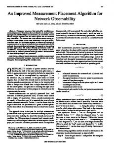
An optimal outcome for any single-objective program (3) lies on the convex upper envelope of outcomes, i.e., the Pareto portion of the boundary of conv(Y ). Such an outcome is said to be supported. Not every Pareto outcome is supported. In fact, the existence of unsupported Pareto outcomes is common in practical problems. Thus, no algorithm that solves (3) for a sequence of values of α can be guaranteed to produce all Pareto outcomes, even in the case where fi is linear for i = 1, 2. A Pareto set for which some outcomes are not supported is illustrated in Figure 1. In the figure, y p and y r are Pareto outcomes, but any convex combination of the two objective functions (linear in the example) produces one of y s , y q , and y t as the optimal outcome. The convex upper envelope of the outcome set is marked by the dashed line. 4

ys

yp

yq

yr yt Figure 1: Example of the convex upper envelope of outcomes. The algorithm of Chalmet et al. [22] searches for Pareto points over subregions of the outcome set. These subregions are generated in such a way as to guarantee that every Pareto point lies on the convex upper envelope of some subregion, ensuring that every Pareto outcome is eventually identified. The algorithm begins by identifying outcomes that maximize y1 and y2 , respectively. Each iteration of the algorithm then searches an unexplored region between two known Pareto points, say y p and y q . The exploration (or probe) consists of solving the problem with a weighted-sum objective and “optimality constraints” that enforce a strict improvement over min{y1p , y1q } and min{y2p , y2q }. If the constrained problem is infeasible, then there is no Pareto outcome in that region. Otherwise the optimal outcome y r is generated and the region is split into the parts between y p and y r and between y r and y q . The algorithm continues until all subregions have been explored in this way. Note that y r need not lie on the convex upper envelope of all outcomes, only of those outcomes between y p and y q , so all Pareto outcomes are generated. Also note that at every iteration, a new Pareto outcome is generated or a subregion is proven empty of outcomes. Thus, the total number of subproblems solved is 2|YE | + 1.

2.2

Weighted Chebyshev Norms

The Chebyshev norm in R2 is the max norm (l∞ norm) defined by kyk∞ = max{|y1 |, |y2 |}. The related distance between two points y 1 and y 2 is d(y 1 , y 2 ) = ky 1 − y 2 k∞ = max{|y11 − y12 |, |y21 − y22 |}.

5

level line for β = .57

ideal point

yp yq level line for β = .29

yr

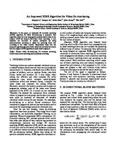
Figure 2: Example of weighted Chebyshev norm level lines. A weighted Chebyshev norm in R2 with weight 0 ≤ β ≤ 1 is defined as k(y1 , y2 )kβ∞ = max{β|y1 |, (1 − β)|y2 |}. The ideal point y ∗ is (y1∗ , y2∗ ) where yi∗ = maxx∈X fi (x) maximizes the single-objective problem with criterion fi . Methods based on weighted Chebyshev norms select outcomes with minimum weighted Chebyshev distance from the ideal point. Figure 2 shows the southwest quadrant of the level lines for two values of β for an example problem. The following are well-known results for the weighted Chebyshev scalarization [73]. Theorem 1 If yˆ ∈ YE is a Pareto outcome, then yˆ solves min{ky − y ∗ kβ∞ } y∈Y

(4)

for some 0 ≤ β ≤ 1. The following result of Bowman [21], used also in [30], was originally stated for the efficient set but it is useful here to state the equivalent result for the Pareto set. Theorem 2 If the Pareto set for (2) is uniformly dominant, then any solution to (4) corresponds to a Pareto outcome. For the remainder of this section, we assume that the Pareto set is uniformly dominant. Techniques for relaxing this assumption are discussed in Section 3.2 and their computational properties are investigated in Section 5.

6

Problem (4) is equivalent to minimize z subject to z ≥ β(y1∗ − y1 ), z ≥ (1 − β)(y2∗ − y2 ), y ∈ Y,

(5)

where 0 ≤ β ≤ 1. As in [30], we partition the set of possible values of β into subintervals over which there is a single unique optimal solution for (5). More precisely, let YE = {y p | p ∈ 1, . . . , N } be the set of Pareto outcomes to (2), ordered so that p < q if and only if y1p < y1q . Under this ordering, y p and y p+1 are called adjacent Pareto points. For any Pareto outcome y p , define βp = (y2∗ − y2p )/(y1∗ − y1p + y2∗ − y2p ),

(6)

and for any pair of Pareto outcomes y p and y q , p < q, define βpq = (y2∗ − y2q )/(y1∗ − y1p + y2∗ − y2q ).

(7)

Equation (7) generalizes the definition of βp,p+1 in [30]. We obtain: 1. For β = βp , y p is the unique optimal outcome for (4), and βp (y1∗ − y1p ) = (1 − βp )(y2∗ − y2p ) = ky ∗ − y p kβ∞ . 2. For β = βpq , y p and y q are both optimal outcomes for (4), and β βpq (y1∗ − y1p ) = (1 − βpq )(y2∗ − y2q ) = ky ∗ − y p kβ∞ = ky ∗ − y q k∞ .

This relationship is illustrated in Figure 3. This analysis is summarized in the following result [30]. Theorem 3 If we assume the Pareto outcomes are ordered so that y11 < y12 < · · · < y1N and y21 > y22 > · · · > y2N then β1 > β12 > β2 > β23 > · · · > βN −1,N > βN . Also, y p is an optimal outcome for (5) with β = βˆ if and only if βp−1,p ≤ βˆ ≤ βp,p+1 . If y p and y q are adjacent outcomes, the quantity βpq is the breakpoint between intervals containing values of β for which y p and y q , respectively, are optimal for (5). Eswaran et al. [30] describe an algorithm for generating the complete Pareto set using a bisection search to approximate the breakpoints. The algorithm begins by identifying an optimal solution to (5) for β = 1 and β = 0. Each iteration searches an unexplored region between pairs of 7

level line for βpq

yp yq

level line for βr yr

Figure 3: Relationship between Pareto points y p , y q , and y r and the weights βr and βpq . consecutive values of β that have been probed so far (say, βp and βq ). The search consists of solving (5) with βp < β = βˆ < βq . If the outcome is y p or y q , then the interval between βˆ and βp or βq , respectively, is discarded. If a new outcome y r is generated, the intervals from βp to βr and from βr to βq are placed on the list to investigate. Intervals narrower than a preset tolerance ξ are discarded. If βˆ = (βp + βq )/2, then the total number of subproblems solved in the worst case is approximately ’ ““ ’ 1 . |YE | 1 + lg (8) (|YE | − 1)ξ Eswaran also describes an interactive algorithm based on pairwise comparisons of Pareto outcomes, but that algorithm can only reach supported outcomes. Solanki [71] proposed an algorithm to generate an approximation to the Pareto set, but that can also be used as an exact algorithm. The algorithm is controlled by an “error measure” associated with each subinterval examined. The error is based on the relative length and width of the unexplored interval. This algorithm also begins by solving (5) for β = 1 and β = 0. Then for each unexplored interval between outcomes y p and y q , a “local ideal point” is (max{y1p , y1q }, max{y2p , y2q }). The algorithm solves (5) with this ideal point and constrained to the region between y p and y q . If no new outcome to this subproblem is found, then the interval is explored completely and its error is zero. Otherwise a new outcome y r is found and the interval is split. The interval with largest error is selected to explore next. The algorithm proceeds until all intervals have error smaller than a preset tolerance. If the error tolerance is zero, this algorithm requires solution of 2|YE | − 1 subproblems and 8

generates the entire Pareto set.

3

An Algorithm for Biobjective Integer Programming

This section describes an improved version of the algorithm of Eswaran et al. [30]. Eswaran’s method has two significant drawbacks: • It cannot be guaranteed to generate all Pareto points if several such outcomes fall in a β-interval of width smaller than the tolerance ξ. If ξ is small enough, then all Pareto outcomes will be found (under the uniform dominance assumption). However, the algorithm does not provide a way to bound ξ to guarantee this result. • As noted above, the running time of the algorithm is heavily dependent on ξ. If ξ is small enough to provide a guarantee that all Pareto outcomes are found, then the algorithm may solve a significant number of subproblems that produce no new information about the Pareto set. Another disadvantage of Eswaran’s algorithm is that it does not generate an exact set of breakpoints. The WCN algorithm generates exact breakpoints, as described in Section 2.2, to guarantee that all Pareto outcomes and the breakpoints are found by solving a sequence of 2|YE | − 1 subproblems. The complexity of our method is on a par with that of Chalmet et al. [22], and the number of subproblems solved is asymptotically optimal. However, as with Eswaran’s algorithm, Chalmet’s method does not generate or exploit the breakpoints. One potential advantage of weighted-sum methods is that they behave correctly in the case of non-uniformly dominant Pareto sets, but Section 3.2.2 describes techniques for dealing with such sets using Chebyshev norms.

3.1

The WCN Algorithm

ˆ be the problem defined by (5) for β = βˆ and let N = |YE |. Then the WCN Let P (β) (weighted Chebyshev norm) algorithm consists of the following steps: Initialization Solve P (1) and P (0) to identify optimal outcomes y 1 and y N , respectively, and the ideal point y ∗ = (y11 , y2N ). Set I = {(y 1 , y N )} and S = {(x1 , y 1 ), (xN , y N )} (where y j = f (xj )). Iteration While I = 6 ∅ do: 1. Remove any (y p , y q ) from I. 2. Compute βpq as in (7) and solve P (βpq ). If the outcome is y p or y q , then y p and y q are adjacent in the list (y 1 , y 2 , . . . , y N ). 3. Otherwise, a new outcome y r is generated. Add (xr , y r ) to S. Add (y p , y r ) and (y r , y q ) to I. By Theorem 3, every iteration of the algorithm must identify either a new Pareto point or a new breakpoint βp,p+1 between adjacent Pareto points. Since the number of breakpoints 9

is N − 1, the total number of iterations is 2N − 1 = O(N ). Any algorithm that identifies all N Pareto outcomes by solving a sequence of subproblems over the set X must solve at least N subproblems, so the number of iterations performed by this algorithm is asymptotically optimal among such methods.

3.2

Algorithmic Enhancements

The WCN algorithm can be improved in a number of ways. We describe some global improvements here. Applications of specialized techniques for the CNRP are described in Section 4. 3.2.1

A Priori Upper Bounds

In step 2, any new outcome y r will have y1r > y1p and y2r > y2q . If no such outcome exists, then the subproblem solver must still re-prove the optimality of y p or y q . In Eswaran’s ˆ determines algorithm, this step is necessary, as which of y p and y q is optimal for P (β) which half of the unexplored interval can be discarded. In the WCN algorithm, generating either y p or y q indicates that the entire interval can be discarded. No additional information is gained by knowing which of y p or y q was generated. Using this fact, the WCN algorithm can be improved as follows. Consider an unexplored interval between Pareto outcomes y p and y q . Let 1 and 2 be positive numbers such that if yr is a new outcome between y p and y q , then yir ≥ min{yip , yiq } + i , for i = 1, 2. For example, if f1 (x) and f2 (x) are integer-valued, then 1 = 2 = 1. Then it must be the case that β β β (9) ky ∗ − y r k∞pq + min{βpq 1 , (1 − βpq )2 } ≤ ky ∗ − y p k∞pq = ky ∗ − y q k∞pq Hence, we can impose an a priori upper bound of β

ky ∗ − y p k∞pq − min{βpq 1 , (1 − βpq )2 }

(10)

when solving the subproblem P (βpq ). This upper bound effectively eliminates all outcomes that do not have strictly smaller Chebyshev norm values from the search space of the subproblem. The outcome of Step 2 is now either a new outcome or infeasibility. Detecting infeasibility generally has a significantly lower computational burden than verifying optimality of a known outcome, so this modification generally improves overall performance. 3.2.2

Relaxing the Uniform Dominance Requirement

Many practical problems (including CNRP) violate the assumption of uniform dominance of the Pareto set made in the WCN algorithm. While probing algorithms based on weighted sums (such as that of Chalmet et al. [22]) do not require this assumption, algorithms based on Chebyshev norms must be modified to take non-uniform dominance into account. If the Pareto set is not uniformly dominant, problem P (β) may have multiple optimal outcomes, some of which are not Pareto. An outcome that is weakly dominated by a Pareto outcome is problematic, because both may lie on the same level line for some weighted Chebyshev norms, hence both may 10

optimal level line

yp

yq yr

Figure 4: Weak domination of y r by y p . solve P (β) for some β encountered in the course of the algorithm. For example, in Figure 4, the dashed rectangle represents the optimal level level of the Chebyshev norm for a given subproblem P (β). In this case, both y p and y q are optimal for P (β), but y p weakly dominates y q . The point y r , which is on a different “edge” of the level line is also optimal, but is neither weakly dominated by nor a weak dominator of either y p or y q . If an outcome y is optimal for some P (β), it must lie on an edge of the optimal level line and cannot be strongly dominated by any other outcome. Solving (5) using a standard branch and bound approach only determines the optimal level line and returns one outcome on that level line. As a secondary objective, we must also ensure that the outcome generated is as close as possible to the ideal point, as measured by an lp norm for some p < ∞. This ensures that the final outcome is Pareto. There are two approaches to this, which we cover in the next two sections. Augmented Chebyshev norms. One way to guarantee that a new outcome found in Step 2 of the WCN algorithm is in fact a Pareto point is to use the augmented Chebyshev norm defined by Steuer [72]. Definition 1 The augmented Chebyshev norm is defined by k(y1 , y2 )kβ,ρ ∞ = max{β|y1 |, (1 − β)|y2 |} + ρ(|y1 | + |y2 |), where ρ is a small positive number. The idea is to ensure that we generate the outcome closest to the ideal point along one edge of the optimal level line, as measured by both the l∞ norm and the l1 norm. This is 11

θ2

augmented level line

yp θ1 yq yr

Figure 5: Augmented Chebyshev norm. Point y p is the unique minimizer of the augmentednorm distance from the ideal point. done by actually adding a small multiple of the l1 norm distance to the Chebyshev norm distance. A graphical depiction of the level lines under this norm is shown in Figure 5. The angle between the bottom edges of the level line is θ1 = tan−1 [ρ/((1 − β + ρ)], and the angle between the left side edges is θ2 = tan−1 [ρ/((β + ρ)]. The problem of determining the outcome closest to the ideal point under this metric is min z + subject to z ≥ z ≥ y ∈

ρ(|y1∗ − y1 | + |y2∗ − y2 |) β(y1∗ − y1 ) (1 − β)(y2∗ − y2 ) Y.

(11)

Because yk∗ − yk ≥ 0 for all y ∈ Y , the objective function can be rewritten as min z − ρ(y1 + y2 ). For fixed ρ > 0 small enough: 12

(12)

• all optimal outcomes for problem (11) are Pareto (in particular, they are not weakly dominated); and • for a given Pareto outcome y for problem (11), there exists 0 ≤ βˆ ≤ 1 such that y is ˆ the unique outcome to problem (11) with β = β. In practice, choosing a proper value for ρ can be problematic. Too small a ρ can cause numerical difficulties because the weight of the secondary objective can lose significance with respect to the primary objective. This situation can lead to generation of weakly dominated outcomes despite the augmented objective. On the other hand, too large a ρ can cause some Pareto outcomes to be unreachable, i.e., not optimal for problem (11) for any choice of β. Steuer [72] recommends 0.001 ≤ ρ ≤ 0.01, but these values are completely ad hoc. The choice of a ρ that works properly depends on the relative size of the optimal objective function values and cannot be computed a priori. In some cases, values of ρ small enough to guarantee detection of all Pareto points (particularly for β close to zero or one) may already be small enough to cause numerical difficulties. Combinatorial methods. An alternative strategy for relaxing the uniform dominance assumption is to implicitly enumerate all optimal outcomes to P (β) and eliminate the weakly dominated ones using cutting planes. This increases the time required to solve P (β), but eliminates the numerical difficulties associated with the augmented Chebyshev norm. To implement this method, the subproblem solver must be allowed to continue to search for alternative optimal outcomes to P (β) and record the best of these with respect to a secondary objective. This is accomplished by modifying the usual pruning rules for the branch and bound algorithm used to solve P (β). In particular, the solver must not prune any node during the search unless it is either proven infeasible or its upper bound falls strictly below that of the best known lower bound, i.e., the best outcome seen so far with respect to the weighted Chebyshev norm. This technique allows alternative optima to be discovered as the search proceeds. An important aspect of this modification is that it includes a prohibition on pruning any node that has already produced an integer feasible solution (corresponding to an outcome in Y ). Although such a solution must be optimal with respect to the weighted Chebyshev norm (subject to the constraints imposed by branching), the outcome may still be weakly dominated. Therefore, when a new outcome yˆ is found, its weighted Chebyshev norm value is compared to that of the best outcome found so far. If the value is strictly larger, the solution is discarded. If the value is strictly smaller, it is installed as the new best outcome seen so far. If its norm value is equal to the current best outcome, it is retained only if it weakly dominates that outcome. After determining whether to install yˆ as the best outcome seen so far, we impose an optimality cut that prevents any outcomes that are weakly dominated by yˆ from being subsequently generated in further processing of the current node. To do so, we determine which of the two constraints z ≥ β(y1∗ − y1 ) z ≥ (1 −

β)(y2∗

13

(13) − y2 )

(14)

from problem (4) is binding at yˆ. This determines on which “edge” of the level line the outcome lies. If only the first constraint is binding, then any outcome y¯ that is weakly dominated by yˆ must have y¯1 < yˆ1 . This corresponds to moving closer to the ideal point in l1 norm distance along the edge of the level line. Therefore, we impose the optimality cut y2 ≥ yˆ2 + 2 ,

(15)

where i is determined as in Section 3.2.1. Similarly, if only the second constraint is binding, we impose the optimality cut y1 ≥ yˆ1 + 1 . (16) If both constraints are binding, this means that the outcome lies at the intersection of the two edges of the level line. In this case, we arbitrarily impose the first cut to try to move along that edge, but if we fail, then we impose the second cut. After imposing the optimality cut, the current outcome becomes infeasible and processing of the node (and possibly its descendants) is continued until either a new outcome is determined or the node proves to be infeasible. One detail we have glossed over is the possibility that the current value of β may be a breakpoint between two previously undiscovered Pareto outcomes. This means there is a distinct outcome on each edge of the optimal level line. In this case, it doesn’t matter which of these outcomes is produced—only that the outcome produced is not weakly dominated. Therefore, once we have found the optimal level line, we confine our search for a Pareto outcome to only one of the edges (the one on which we discover a solution first). This is accomplished by discarding any outcome discovered that has the same weighted Chebyshev norm value as the current best, but is incomparable to it, i.e., is neither weakly dominated by nor a weak dominator of it. Hybrid methods. A third alternative, which is effective in practice, is to combine the augmented Chebyshev norm method with the combinatorial method described above. To do so, we simply use the augmented objective function (12) while also applying the combinatorial methodology described above. This has the effect of guarding against values of ρ that are too small to ensure generation of Pareto outcomes, while at the same time guiding the search toward Pareto outcomes. In practice, this hybrid method tends to reduce running times over the pure combinatorial method. Computational results with both methods are presented in Section 5.

3.3

Approximation of the Pareto Set

If the number of Pareto outcomes is large, the computational burden of generating the entire set may be unacceptable. In that case, it may be desirable to generate just a subset of representative points, where a “representative” subset is one that is “well-distributed over the entire set” [71]. Deterministic algorithms using Chebyshev norms have been proposed to accomplish that task for general multicriteria programs that subsume BIPs [47, 50, 52], but the works of Solanki [71] and Schandl et al. [69] seem to be the only specialized deterministic algorithms proposed for BIPs. None of the papers known to the authors offer in-depth

14

computational results on the approximation of the Pareto set of BIPs with deterministic algorithms (see Ruzika and Wiecek [68] for a recent review). Solanki’s method minimizes a geometric measure of the “error” associated with the generated subset of Pareto outcomes, generating the smallest number of outcomes required to achieve a prespecified bound on the error. Schandl’s method employs polyhedral norms not only to find an approximation but also to evaluate its quality. A norm method is used to generate supported Pareto outcomes while the lexicographic Chebyshev method and a cutting-plane approach are proposed to find unsupported Pareto outcomes. Any probing algorithm can generate an approximation to the Pareto set by simply terminating early. (Solanki’s algorithm can generate the entire Pareto set by simply running until the error measure is zero.) The representativeness of the resulting approximation can be influenced by controlling the order in which available intervals are selected for exploration. Desirable features for such an ordering are: • the points should be representative, and • the computational effort should be minimized. In the WCN algorithm, both of these goals are advanced by selecting unexplored intervals in a first-in-first-out (FIFO) order. FIFO selection increases the likelihood that a subproblem results in a new Pareto outcome and tends to minimize the number of infeasible subproblems, i.e., probes that don’t generate new outcomes, when terminating the algorithm early. It also tends to distribute the outcomes across the full range of β. Section 5 describes a computational experiment demonstrating this result.

3.4

An Interactive Variant of the Algorithm

After employing an algorithm to find all (or a large subset of) Pareto outcomes, a decision maker intending to use the results of such an algorithm must then engage in a second phase of decision making to determine the one Pareto point that best suits the needs of the organization. In order to select the “best” from among a set of Pareto outcomes, the outcomes must ultimately be compared with respect to a single-objective utility function. If the decision maker’s utility function is known, then the final outcome selection can be made automatically. Determining the exact form of this utility function for a particular decision maker, however, is a difficult challenge for researchers. The process usually involves restrictive assumptions on the form of such a utility function, and may require complicated input from the decision maker. An alternative strategy is to allow the decision maker to search the space of Pareto outcomes interactively, responding to the outcomes displayed by adjusting parameters to direct the search toward more desirable outcomes. An interactive version of the WCN algorithm consists of the following steps: Initialization Solve P (1) and P (0) to identify optimal outcomes y 1 and y N , respectively, and the ideal point y ∗ = (y11 , y2N ). Set I = {(y 1 , y N )} and S = {(x1 , y 1 ), (xN , y N )} (where y j = f (xj )). Iteration While I = 6 ∅ do: 15

1. Allow user to select (y p , y q ) from I. Stop if user declines to select. Compute βpq as in (7) and solve P (βpq ). 2. If no new outcome is found, then y p and y q are adjacent in the list (y 1 , y 2 , . . . , y N ). Report this fact to the user. 3. Otherwise, a new outcome y r is generated. Report (xr , y r ) to the user and add it to S. Add (y p , y r ) and (y r , y q ) to I. This algorithm can be used as an interactive “binary search,” in which the decision maker evaluates a proposed outcome and decides whether to give up some value with respect to the first objective in order to gain some value in the second or vice versa. If the user chooses to sacrifice with respect to objective f1 , the next probe finds an outcome (if one exists) that is better with respect to f1 than any previously-identified outcome except the last. In this way, the decision maker homes in on a satisfactory outcome or on a pair of adjacent outcomes that is closest to the decision maker’s preference. Unlike many interactive algorithms, this one does not attempt to model the decision maker’s utility function. Thus, it makes no assumptions regarding the form of this function and neither requires nor estimates parameters of the utility function.

3.5

Analyzing Tradeoff Information

In interactive algorithms, it can be helpful for the system to provide the decision maker with information about the tradeoff between objectives in order to aid the decision to move from a candidate outcome to a nearby one. In problems where the boundary of the Pareto set is continuous and differentiable, the slope of the tangent line associated with a particular outcome provides local information about the rate at which the decision maker trades off value between objective functions when moving to nearby outcomes. With discrete problems, there is no tangent line to provide local tradeoff information. Tradeoffs between a candidate outcome and another particular outcome can be found by computing the ratio of improvement in one objective to the decrease in the other. This information, however, is specific to the outcomes being compared and requires knowledge of both outcomes. In addition, achieving the computed tradeoff requires moving to the particular alternate outcome used in the computation, perhaps bypassing intervening outcomes (in the ordering of Theorem 3) or stopping short of more distant ones with different (higher or lower) tradeoff rates. A global view of tradeoffs for continuous Pareto sets, based on the pairwise comparison described above, is provided by Kaliszewski [44]. For a decrease in one objective, the tradeoff with respect to the other is the supremum of the ratio of the improvement to the decrease over all outcomes that actually decrease the first objective and improve the second. Kaliszewski’s technique can be extended to discrete Pareto sets, as follows. With respect to a particular outcome y p , a pairwise tradeoff between y p and another outcome y q with respect to objectives i and j is defined as Tij (y p , y q ) =

16

yiq − yip . yjp − yjq

yp

G (y p ) and T G (y p ) illustrated. Figure 6: Tradeoff measures T12 21

Note that Tji (y p , y q ) = Tij (y p , y q )−1 . In comparing Pareto outcomes, we adopt the convention that objective j is the one that decreases when moving from y p to y q , so the denominator is positive and the tradeoff is expressed as units of increase in objective i per unit decrease in objective j. Then a global tradeoff with respect to y p when allowing decreases in objective j is given by yi − yip . TijG (y p ) = max p p y∈Y :yj yˆij }. The difficulty is in finding the set S. In our implementation, S is found using greedy procedures exactly analogous to those used for locating violated GSECs. Beginning with a randomly selected kernel, the set is grown greedily by adding one customer at a time in such a way that the violation of the new inequality increases. This continues until no new customer can be added. Flow cover inequalities. In addition to the problem-specific inequalities listed above, we also generate flow cover inequalities. These are well-known to be effective on problems with variable upper bounds, such as FCNFPs and CNRPs. A description of this class of inequalities, as well as separation methods is contained in [78]. The implementation used was developed by Xu [79] and is available from the COIN-OR Cut Generator Library [54].

4.4

Customizing SYMPHONY

We implemented our branch and cut algorithm using a framework for parallel branch, cut, and price (BCP) called SYMPHONY [63]. SYMPHONY achieves a “black box” structure by separating the problem-specific methods from the rest of the implementation. The internal library interfaces with the user’s subroutines through a well-defined API and independently performs all the normal functions of BCP—tree management, LP solution, and pool management, as well as inter-process communication (when parallelism is employed). Although there are default options for all operations, the user can assert control over the behavior of the algorithm by overriding the default methods and through a myriad of parameters. Implementation of the solver consisted mainly of writing custom user subroutines to modify the default of behavior of SYMPHONY. Eliminating weakly dominated outcomes. To eliminate weakly dominated outcomes, we used the hybrid method described in Section 3.2.2. To accommodate this method, we modified the SYMPHONY framework itself to allow the user to specify that the search should continue despite having found a feasible solution at a particular search tree node (see Section 3.2.2). The task of tracking the best outcome seen so far and imposing the optimality cuts is still left to the user for now. In the future, we hope to build this feature into the SYMPHONY framework. SYMPHONY also has a parameter called “granularity” that must be adjusted. The granularity is a constant that gets subtracted from the value of the current incumbent solution to determine the cutoff for pruning nodes during the search. For instance, for integer programs with integral objective function coefficients, this parameter can be set to 1, which means that any node whose bound is not at least one unit better than the best solution seen so far can be pruned. To enumerate all alternative optimal solutions, we set this parameter to −, where  was a value between the zero tolerance and the minimum difference in Chebyshev norm values between an outcome and any weak dominator of that outcome (see more discussion in the paragraph on tolerances below), so that no node would be pruned until its bound was strictly worse the value of the current best outcome. 22

Cut generation. The main job in implementing the solver consisted of writing custom routines to do problem-specific cut generation. Our overall approach to separation was straightforward. As described earlier, we left the flow capacity constraints and the edge cuts out of the formulation and generated those dynamically. If inequalities in either of these classes were found, then cut generation ceased for that iteration. If no inequalities of either of these classes were found, then we attempted to generate mixed dicut inequalities. Flow cover inequalities, as well as other classes of inequalities valid for generic mixed-integer programs are automatically generated by SYMPHONY using COIN-OR’s cut generation library [54]. This is done in every iteration by default. SYMPHONY also includes a global cut pool in which previously generated cuts can be stored for later use. We utilized the pool for storing cuts both for use during the solution of the current subproblem and for later use during solution of subsequent subproblems. Because they are so easy to generate, we did not store either flow capacity constraints or edge cuts. Also, we could not store flow cover inequalities, since these are generally not globally valid. Therefore, we only used the cut pool to store the mixed dicut inequalities. By default, these inequalities were only sent to the pool after they had remained binding in the LP relaxation for at least three iterations. The cuts in the pool were dynamically ordered by a rolling average degree of violation so that the “most important” cuts (by this measure) were always at the top of the list. During each call to the cut pool, only cuts near the top of the list were checked for violation. To take advantage of optimizing over the same feasible region repeatedly, we retained the cut pool between subproblems, so that the calculation could be warm-started with good cuts found solving previous subproblems. Branching. For branching, we used SYMPHONY’s built-in strong branching facility and selected fixed-charge variables whose values were closest to .5 as the candidates. Empirically, seven candidates seemed to be a good number for these problems. SYMPHONY allows for a gradual reduction in the number of candidates at deeper levels of the tree, but we did not use this facility. Other customizations. We wrote a customized engine for parsing the input files (which use slight modifications of the TSPLIB format) and generating the formulation. SYMPHONY allows the user to specify a set of core variables, which are considered to have an increased probability of participating in an optimal solution. We defined the core variables to be those corresponding to the edges in a sparse graph generated by taking the k shortest edges incident to each node in the original graph. Error tolerances and other parameters. Numerical issues are particularly important when implementing algorithms for enumerating Pareto outcomes. To deal with numerical issues, it was necessary to define a number of different error tolerances. As always, we had an integer tolerance for determining whether a given variable was integer valued or not. For this value, we used SYMPHONY’s internal error tolerance, which in turn depends on the LP solver’s error tolerance. We also had to specify the minimum Chebyshev norm distance between any two distinct outcomes. Although the CNRP has continuous variables, it is easy 23

to show that there always exists an integer optimal solution as long as the demands are integral. Thus, this parameter could be set to 1. From this parameter and the parameter β, we determined the minimum difference in the value of the weighted Chebyshev norm for two outcomes, one of which weakly dominates the other. This was used as the granularity mentioned above. We also specified the weight ρ for the secondary objective in the augmented Chebyshev norm method. Selection of this parameter value is discussed below. Finally, we had to specify a tolerance for performing the bisection method of Eswaran. Selection of this tolerance is also discussed below.

5 5.1

Computational Study Setup

Because solving a single instance of the FCNFP is already very difficult, we needed a test set containing instances small enough to be solved repeatedly in reasonable time but still challenging enough to be interesting. Instances of the VRP are a natural candidates because they come with a prespecified central node as well as customer demand and capacity data, although the latter are unnecessary for specifying a CTP instance. We took Euclidean instances from the library of VRP instances maintained by author Ralphs [62] and randomly sampled from among the customer nodes to obtain problems with between 10 and 20 customers. The 10-customer problems were typically easy and a few of the 20-customer problems were extremely difficult, so we confine our reporting to the 15-customer problems constructed in this way. The test set had enough variety to make reasonably broad conclusions about the methods that are the subject of this study. The computational platform was an SMP machine with four Intel Xeon 700MHz CPUs and 2G of memory (memory was never an issue). These experiments were performed with a slightly modified version of SYMPHONY 4.0. SYMPHONY is designed to work with a number of LP solvers through the COIN-OR Open Solver Interface. For the runs reported here, we used the OSI CPLEX interface with CPLEX 8.1 as the underlying LP solver. In designing the computational experiments, there were several comparisons we wanted to make. First, we wanted to compare our exact approach to the bisection algorithm of Eswaran in terms of both computational efficiency and ability to produce all Pareto outcomes. Second, we wanted to compare the various approaches described in Section 3.2.2 for relaxing the uniform dominance assumption. Third, we wanted to test various approaches to approximating the set of Pareto outcomes. The results of these experiments are described in the next section.

5.2

Results

We report here on four experiments, each described in a separate table. In each table, the methods are compared to the WCN method (plus optimality cuts and the combinatorial method for eliminating weakly dominated outcomes), which is used as a baseline. All numerical data are reported as differences from the baseline method to make it easier to spot trends. On each chart, the group of columns labeled Iterations gives the total number of subproblems solved. The column labeled Outcomes Found gives the total number of Pareto 24

outcomes reported by the algorithm. The Max Missed column contains the maximum number of missing Pareto outcomes in any interval between two Pareto outcomes that were found. This is a rough measure of how the missing Pareto outcomes are distributed among the found outcomes, and therefore indicates how well distributed the found outcomes are among the set of all Pareto outcomes. The entries in these columns in the Totals row are arithmetic means. Finally, the column labeled CPU seconds is the running time of the algorithm on the platform described earlier. In Table 1, we compare the WCN algorithm to the bisection search algorithm of Eswaran for three different tolerances, ξ = 10−1 , 10−2 , and 10−3 . Note that our implementation of Eswaran’s algorithm uses the approach described in Section 3.2.2 for eliminating weakly dominated outcomes. Even at a tolerance of 10−3 some outcomes are missed for the instance att48, which has a number of small nonconvex regions in its frontier. It is clear that the tradeoff between tolerance and running time favors the WCN algorithm for this test set. The tolerance required in order to have a reasonable expectation of finding the full set of Pareto outcomes results in a running time far exceeding that for the WCN algorithm. This is predictable, based on the crude estimate of the number of iterations required in the worst case for Eswaran’s algorithm given by (8) and we expect that this same behavior would hold for most classes of BIPs. In Table 2, we compare the WCN algorithm with the ACN method described in Section 3.2.2 (i.e., the WCN method with augmented Chebyshev norms). Here, the columns are labeled with the secondary objective function weight ρ that was used. Although the ACN method is much faster for large secondary objective function weights (as one would expect), the results demonstrate why it is not possible in general to determine a weight for the secondary objective function that both ensures the enumeration of all Pareto outcomes and protects against the generation of weakly dominated outcomes. Note that for ρ = 10−4 , the ACN algorithm generates more outcomes than the WCN (which generates all Pareto outcomes) for instances A-n33-k6 and B-n43-k6. This is because the ACN algorithm is producing weakly dominated outcomes in these cases, due to the value of ρ being set too small. Even setting the tolerance separately for each instance does not have the desired effect, as there are several other instances for which the algorithm both produced one more or more weakly dominated outcomes and missed Pareto outcomes. For these instances, no tolerance will work properly. In Table 3, we compare WCN to the hybrid algorithm also described in Section 3.2.2. The value of ρ used is displayed above the columns of results for the hybrid algorithm. As described earlier, the hybrid algorithm has the advantages of both the ACN and the WCN algorithms and allows ρ to be set small enough to ensure correct behavior. As expected, the table shows that as ρ decreases, running times for the hybrid algorithm increase. However, it appears that choosing ρ approximately 10−5 results in a reduction in running time without a great loss in terms of accuracy. We also tried setting ρ to 10−6 and in this case, the full Pareto set is found for every problem, but the advantage in terms of running time is insignificant. Finally, we experimented with a number of approximation methods. As discussed in Section 3.3, we chose to judge the performance of the various heuristics on the basis of both running time and the distribution of outcomes found among the entire set, as measured by 25

the maximum number of missed outcomes in any interval between found outcomes. The results described in Table 1 indicate that Eswaran’s bisection algorithm does in fact make a good heuristic based on our measure of distribution of outcomes, but the reduction in running times doesn’t justify the loss of accuracy. The ACN algorithm with a relatively large value of ρ also makes a reasonable heuristic and the running times are much better. One disadvantage of these two methods is that it would be difficult to predict a priori the behavior of these algorithms, both in terms of running time and number of Pareto outcomes produced. To get a predictable number of outcomes in a predictable amount of time, we simply stopped the WCN algorithm after a fixed number of outcomes had been produced. The distribution of the resulting set of outcomes depends largely on the order in which the outcome pairs are processed, so we compared a FIFO ordering to a LIFO ordering. One would expect the FIFO ordering, which prefers processing parts of outcomes that are “far apart” from each other, to outperform the LIFO ordering, which prefers processing pairs of outcomes that are closer together. Table 4 shows that this is in fact the case. In these experiments, we stopped the algorithm after 15 outcomes were produced (the table only includes problems with more than 15 Pareto outcomes). The distribution of outcomes for the FIFO algorithm is dramatically better than that for the LIFO algorithm. Of course, other orderings are also possible. We also tried generating supported outcomes as a possible heuristic approach. This can be done extremely quickly, but the quality of the sets of outcomes produced was very low.

6

Conclusion

We have described an algorithm for biobjective discrete programs (BIPs) based on weighted Chebyshev norms. The algorithm improves on the similar method of Eswaran et al. [30] by providing a guarantee that all Pareto outcomes are identified and with a minimum number of solutions of scalarized subproblems. The method thus matches the complexity of the best methods available for such problems. It also extends naturally to approximation of the Pareto set and to nonparametric interactive applications. We have described an extension of a global tradeoff analysis technique to discrete problems. We implemented the algorithm in the SYMPHONY branch-cut-price framework and demonstrated that it performs effectively on a class of network routing problems. Topics for future research include incorporation of the method into the open-source SYMPHONY framework and study of the performance of a parallel implementation of the WCN algorithm.

7

Acknowledgments

Authors Saltzman and Wiecek were partially supported by ONR Grant N00014-97-1-0784.

26

27

Name eil13 E-n22-k4 E-n23-k3 E-n30-k3 E-n33-k4 att48 E-n51-k5 A-n32-k5 A-n33-k5 A-n33-k6 A-n34-k5 A-n36-k5 A-n37-k5 A-n38-k5 A-n39-k5 A-n39-k6 A-n45-k6 A-n46-k7 B-n31-k5 B-n34-k5 B-n35-k5 B-n38-k6 B-n39-k5 B-n41-k6 B-n43-k6 B-n44-k7 B-n45-k5 B-n50-k7 B-n51-k7 B-n52-k7 B-n56-k7 B-n64-k9 A-n48-k7 A-n53-k7 Totals

CPU sec WCN ∆ from WCN −1 0 10 10−2 10−3 1.67 0.80 3.66 6.92 133.92 −14.39 60.62 286.73 159.93 11.81 77.38 333.16 38.58 6.10 26.35 82.00 711.19 110.45 475.79 1828.89 83.67 −24.51 −2.75 83.96 28.20 −3.69 4.93 32.51 91.09 −14.39 48.88 205.81 47.92 5.33 17.85 86.66 174.06 −12.97 84.87 371.72 34.39 −8.61 18.20 62.49 91.53 18.26 43.22 172.02 51.72 −10.96 27.27 82.67 12.74 −2.50 7.98 18.45 150.10 −4.08 77.08 280.35 43.58 −12.32 14.21 60.79 63.73 −0.05 18.54 107.43 31.56 −10.41 3.01 43.63 1269.31 65.10 482.66 2549.87 1634.27 −432.33 156.30 2323.22 1622.09 −686.11 209.55 2319.96 315.14 65.12 101.43 659.89 89.78 −21.91 13.31 121.77 280.88 −30.58 103.86 618.33 206.18 −121.97 77.76 380.82 70.40 15.43 68.85 209.81 36.58 −0.15 12.88 54.92 75.11 −9.82 22.25 122.58 93.61 −27.64 43.86 168.38 70.85 10.69 29.00 117.64 62.55 −13.33 12.65 83.27 139.14 −32.42 20.31 200.32 171.70 −24.42 29.13 299.72 118.86 −12.49 35.06 227.27 8206.03 −1222.96 2425.95 14603.96 Table 1: Comparing the WCN Algorithm with Bisection Search

Iterations Solutions Found Max Missed WCN ∆ from WCN WCN ∆ from WCN 0 10−1 10−2 10−3 0 10−1 10−2 10−3 10−1 10−2 10−3 11 4 17 32 6 0 0 0 0 0 0 79 −8 23 132 40 −4 0 0 1 0 0 107 −8 18 150 54 −4 0 0 1 0 0 45 1 25 86 23 0 0 0 0 0 0 85 −4 24 142 43 −2 0 0 1 0 0 147 −35 −9 104 74 −18 −15 −4 3 3 1 57 −2 27 111 29 −1 0 0 1 0 0 75 −12 24 114 38 −6 −1 0 2 1 0 65 −4 23 105 33 −2 −1 0 1 1 0 77 −6 21 124 39 −3 0 0 1 0 0 37 −8 26 78 19 −4 0 0 1 0 0 91 −2 22 134 46 −1 0 0 1 0 0 65 −10 24 104 33 −5 0 0 2 0 0 25 −4 25 61 13 −2 0 0 1 0 0 79 −10 26 127 40 −5 0 0 1 0 0 55 −8 26 101 28 −4 0 0 2 0 0 77 −8 21 124 39 −4 −1 0 1 1 0 67 −10 22 117 34 −5 0 0 2 0 0 109 −4 18 155 55 −2 0 0 1 0 0 127 −24 15 151 64 −12 −1 0 4 1 0 75 −24 20 108 38 −12 −2 0 2 1 0 79 −2 22 122 40 −1 −1 0 1 1 0 63 −6 22 112 32 −3 −1 0 1 1 0 73 −18 20 112 37 −9 0 0 3 0 0 69 −12 25 112 35 −6 −1 0 5 1 0 51 −6 26 95 26 −3 0 0 1 0 0 63 −2 25 112 32 −1 0 0 1 0 0 79 −12 21 125 40 −6 −1 0 1 1 0 51 −7 18 82 26 −4 0 0 2 0 0 91 −8 20 137 46 −4 0 0 2 0 0 61 −2 26 112 31 −1 0 0 1 0 0 89 −8 20 140 45 −4 0 0 1 0 0 115 −22 15 140 58 −11 −2 0 3 1 0 89 −8 17 137 45 −4 −1 0 1 1 0 2528 −299 715 3898 1281 −153 −28 −4 1 0 0

28

Name eil13 E-n22-k4 E-n23-k3 E-n30-k3 E-n33-k4 att48 E-n51-k5 A-n32-k5 A-n33-k5 A-n33-k6 A-n34-k5 A-n36-k5 A-n37-k5 A-n38-k5 A-n39-k5 A-n39-k6 A-n45-k6 A-n46-k7 B-n31-k5 B-n34-k5 B-n35-k5 B-n38-k6 B-n39-k5 B-n41-k6 B-n43-k6 B-n44-k7 B-n45-k5 B-n50-k7 B-n51-k7 B-n52-k7 B-n56-k7 B-n64-k9 A-n48-k7 A-n53-k7 Totals

WCN 0 1.67 133.92 159.93 38.58 711.19 83.67 28.20 91.09 47.92 174.06 34.39 91.53 51.72 12.74 150.10 43.58 63.73 31.56 1269.31 1634.27 1622.09 315.14 89.78 280.88 206.18 70.40 36.58 75.11 93.61 70.85 62.55 139.14 171.70 118.86 8206.03 Table 2: Comparing the WCN Algorithm with the ACN Algorithm

Iterations Solutions Found Max Missed WCN ∆ from WCN WCN ∆ from WCN 0 10−2 10−3 10−4 0 10−2 10−3 10−4 10−2 10−3 10−4 11 −6 0 0 6 −3 0 0 2 0 0 79 −68 −22 0 40 −34 −11 0 10 2 0 107 −96 −52 −4 54 −48 −26 −2 13 5 1 45 −38 −16 0 23 −19 −8 0 8 2 0 85 −76 −44 −2 43 −38 −22 −1 12 4 1 147 −140 −106 −62 74 −70 −53 −31 44 17 8 57 −46 −10 0 29 −23 −5 0 8 1 0 75 −62 −36 −2 38 −31 −18 −1 13 4 1 65 −52 −22 −2 33 −26 −11 −1 9 3 1 77 −66 −28 2 39 −33 −14 1 12 2 0 37 −30 −10 0 19 −15 −5 0 6 1 0 91 −82 −42 0 46 −41 −21 0 13 4 0 65 −54 −22 0 33 −27 −11 0 12 2 0 25 −16 −4 0 13 −8 −2 0 3 1 0 79 −70 −34 −2 40 −35 −17 −1 13 3 1 55 −44 −16 0 28 −22 −8 0 10 2 0 77 −68 −34 0 39 −34 −17 0 12 2 0 67 −58 −28 −4 34 −29 −14 −2 9 2 1 109 −98 −58 0 55 −49 −29 0 14 3 0 127 −114 −64 −8 64 −57 −32 −4 18 4 1 75 −66 −42 0 38 −33 −21 0 11 4 1 79 −68 −40 −2 40 −34 −20 −1 10 4 1 63 −52 −20 −2 32 −26 −10 −1 9 3 1 73 −64 −34 0 37 −32 −17 0 11 4 0 69 −58 −26 2 35 −29 −13 1 9 3 0 51 −42 −16 0 26 −21 −8 0 8 2 0 63 −54 −26 0 32 −27 −13 0 7 2 0 79 −70 −32 −2 40 −35 −16 −1 12 3 1 51 −42 −26 0 26 −21 −13 0 8 3 0 91 −82 −42 −2 46 −41 −21 −1 15 3 1 61 −54 −22 0 31 −27 −11 0 14 2 1 89 −80 −38 −4 45 −40 −19 −2 12 3 1 115 −102 −66 −2 58 −51 −33 −1 17 3 1 89 −78 −40 0 45 −39 −20 0 12 4 0 2528 −2196 −1118 −96 1281 −1098 −559 −48 11 3 0

CPU sec ∆ from WCN −2 10 10−3 10−4 −1.40 −0.62 −0.46 −122.65 −58.56 −5.94 −147.46 −115.04 −48.62 −36.79 −27.24 −6.20 −686.94 −544.82 −142.95 −80.14 −59.83 −28.48 −26.10 −15.44 −2.33 −73.62 −64.93 −18.27 −43.45 −24.40 −2.32 −164.15 −102.49 −28.56 −32.05 −20.42 −5.85 −83.96 −52.93 −13.26 −45.02 −22.97 −5.19 −11.54 −8.00 −2.57 −141.80 −103.96 −38.25 −39.14 −26.16 −4.66 −59.31 −36.43 −2.45 −29.00 −20.87 −7.21 −1233.36 −907.48 −269.72 −1541.35 −1210.95 −281.50 −1573.85 −805.70 −368.15 −307.12 −204.21 −20.09 −82.14 −49.02 −27.21 −269.08 −174.53 −27.31 −198.45 −151.42 −45.29 −64.49 −28.54 −7.50 −33.57 −22.16 5.12 −67.22 −37.62 −5.59 −88.43 −66.91 −2.56 −66.55 −34.46 1.81 −60.44 −39.26 −14.47 −130.77 −73.08 −16.01 −159.07 −129.36 −35.29 −108.24 −64.56 −2.52 −7808.65 −5304.37 −1479.85

29

Name eil13 E-n22-k4 E-n23-k3 E-n30-k3 E-n33-k4 att48 E-n51-k5 A-n32-k5 A-n33-k5 A-n33-k6 A-n34-k5 A-n36-k5 A-n37-k5 A-n38-k5 A-n39-k5 A-n39-k6 A-n45-k6 A-n46-k7 B-n31-k5 B-n34-k5 B-n35-k5 B-n38-k6 B-n39-k5 B-n41-k6 B-n43-k6 B-n44-k7 B-n45-k5 B-n50-k7 B-n51-k7 B-n52-k7 B-n56-k7 B-n64-k9 A-n48-k7 A-n53-k7 Totals

CPU sec WCN ∆ from WCN −3 0 10 10−4 10−5 1.67 −0.59 −0.43 −0.41 133.92 −59.40 6.63 16.09 159.93 −111.13 −52.20 −18.32 38.58 −26.47 −3.31 6.41 711.19 −557.64 −117.01 −44.50 83.67 −59.34 −30.19 −1.12 28.20 −15.03 −0.88 0.25 91.09 −66.46 −16.45 −2.75 47.92 −25.97 −6.81 1.63 174.06 −94.31 −16.14 −16.60 34.39 −19.42 −6.71 0.81 91.53 −49.28 −7.28 3.27 51.72 −22.66 −0.93 −0.22 12.74 −7.97 −2.55 −0.38 150.10 −99.51 −39.95 −24.69 43.58 −22.58 −10.06 −3.64 63.73 −34.80 −7.19 0.21 31.56 −20.73 −7.41 −2.23 1269.31 −931.70 −259.41 −14.80 1634.27 −1243.75 −332.76 −107.81 1622.09 −974.89 −441.89 −349.88 315.14 −221.02 −49.37 −21.84 89.78 −56.63 −19.80 −10.11 280.88 −178.82 −40.61 −8.72 206.18 −150.86 −30.41 −10.28 70.40 −33.05 −3.90 −0.91 36.58 −22.65 3.59 8.19 75.11 −33.21 −6.45 9.99 93.61 −66.59 −12.29 −8.39 70.85 −35.33 1.87 8.66 62.55 −36.17 −7.50 −3.96 139.14 −72.10 −4.31 3.93 171.70 −129.44 −34.75 −1.39 118.86 −61.37 −4.68 2.49 8206.03 −5540.87 −1561.54 −591.02

Table 3: Comparing the WCN Algorithm with the Hybrid ACN Algorithm

Iterations Solutions Found Max Missed WCN ∆ from WCN WCN ∆ from WCN 0 10−3 10−4 10−5 0 10−3 10−4 10−5 10−3 10−4 10−5 11 0 0 0 6 0 0 0 0 0 0 79 −22 0 0 40 −11 0 0 2 0 0 107 −52 −4 0 54 −26 −2 0 5 1 0 45 −16 0 0 23 −8 0 0 2 0 0 85 −44 −2 0 43 −22 −1 0 4 1 0 147 −106 −62 −6 74 −53 −31 −3 17 8 2 57 −10 0 0 29 −5 0 0 1 0 0 75 −36 −2 0 38 −18 −1 0 4 1 0 65 −22 −2 0 33 −11 −1 0 3 1 0 77 −28 0 0 39 −14 0 0 2 0 0 37 −10 0 0 19 −5 0 0 1 0 0 91 −42 0 0 46 −21 0 0 4 0 0 65 −22 0 0 33 −11 0 0 2 0 0 25 −4 0 0 13 −2 0 0 1 0 0 79 −34 −2 0 40 −17 −1 0 3 1 0 55 −16 0 0 28 −8 0 0 2 0 0 77 −34 0 0 39 −17 0 0 2 0 0 67 −28 −4 0 34 −14 −2 0 2 1 0 109 −58 0 0 55 −29 0 0 3 0 0 127 −64 −10 −2 64 −32 −5 −1 4 1 1 75 −42 −2 0 38 −21 −1 0 4 1 0 79 −40 −2 0 40 −20 −1 0 4 1 0 63 −20 −2 0 32 −10 −1 0 3 1 0 73 −34 0 0 37 −17 0 0 4 0 0 69 −26 0 0 35 −13 0 0 3 0 0 51 −16 0 0 26 −8 0 0 2 0 0 63 −26 0 0 32 −13 0 0 2 0 0 79 −32 −2 0 40 −16 −1 0 3 1 0 51 −26 0 0 26 −13 0 0 3 0 0 91 −42 −2 0 46 −21 −1 0 3 1 0 61 −22 −2 0 31 −11 −1 0 2 1 0 89 −38 −4 0 45 −19 −2 0 3 1 0 115 −66 −2 0 58 −33 −1 0 3 1 0 89 −40 0 0 45 −20 0 0 4 0 0 2528 −1118 −106 −8 1281 −559 −53 −4 3 0 0

30

Name E-n22-k4 E-n23-k3 E-n30-k3 E-n33-k4 att48 E-n51-k5 A-n32-k5 A-n33-k5 A-n33-k6 A-n34-k5 A-n36-k5 A-n37-k5 A-n39-k5 A-n39-k6 A-n45-k6 A-n46-k7 B-n31-k5 B-n34-k5 B-n35-k5 B-n38-k6 B-n39-k5 B-n41-k6 B-n43-k6 B-n44-k7 B-n45-k5 B-n50-k7 B-n51-k7 B-n52-k7 B-n56-k7 B-n64-k9 A-n48-k7 A-n53-k7 Totals 133.92 159.93 38.58 711.19 83.67 28.20 91.09 47.92 174.06 34.39 91.53 51.72 150.10 43.58 63.73 31.56 1269.31 1634.27 1622.09 315.14 89.78 280.88 206.18 70.40 36.58 75.11 93.61 70.85 62.55 139.14 171.70 118.86 8191.62

WCN

CPU sec ∆ from WCN FIFO LIFO −101.23 −104.61 −132.99 −130.12 −27.54 −17.79 −594.79 −671.83 −69.08 −73.55 −18.78 −20.38 −58.33 −75.49 −31.56 −31.35 −123.99 −141.08 −14.95 −12.84 −70.76 −63.59 −34.25 −35.39 −96.56 −93.22 −25.83 −28.23 −47.24 −48.09 −19.88 −23.65 −1114.98 −1186.93 −1411.45 −1510.76 −957.94 −1562.38 −249.31 −290.48 −63.20 −68.17 −224.22 −236.91 −135.88 −163.67 −50.15 −41.08 −25.25 −20.52 −50.87 −50.97 −46.19 −74.53 −55.38 −59.48 −42.92 −36.02 −99.47 −121.41 −141.26 −151.12 −87.90 −98.91 −6224.13 −7244.55

Table 4: Comparing Limited WCN Algorithm with LIFO and FIFO Ordering

79 107 45 85 147 57 75 65 77 37 91 65 79 55 77 67 109 127 75 79 63 73 69 51 63 79 51 91 61 89 115 89 2492

WCN

Iterations Solutions Found Max Missed ∆ from WCN WCN ∆ from WCN FIFO LIFO FIFO LIFO FIFO LIFO −64 −55 40 −25 −25 4 18 −92 −83 54 −39 −39 6 27 −29 −19 23 −8 −8 3 8 −70 −61 43 −28 −28 4 23 −132 −128 74 −59 −59 23 24 −41 −33 29 −14 −14 4 10 −60 −51 38 −23 −23 10 11 −50 −40 33 −18 −18 5 11 −62 −52 39 −24 −24 6 12 −19 −11 19 −4 −4 1 2 −76 −68 46 −31 −31 7 15 −50 −40 33 −18 −18 6 13 −64 −55 40 −25 −25 8 13 −39 −29 28 −13 −13 5 7 −62 −51 39 −24 −24 5 22 −52 −42 34 −19 −19 4 12 −94 −83 55 −40 −40 7 29 −112 −103 64 −49 −49 9 32 −60 −49 38 −23 −23 4 22 −64 −55 40 −25 −25 4 22 −47 −39 32 −17 −17 3 11 −58 −49 37 −22 −22 6 20 −54 −44 35 −20 −20 5 10 −36 −27 26 −11 −11 3 8 −48 −38 32 −17 −17 3 15 −64 −54 40 −25 −25 5 20 −35 −27 26 −11 −11 3 7 −76 −65 46 −31 −31 7 30 −46 −35 31 −16 −16 3 14 −74 −65 45 −30 −30 7 22 −100 −92 58 −43 −43 11 20 −73 −66 45 −30 −30 7 19 −2003 −1709 1262 −782 −782 6 17

References [1] Y. Aksoy. An interactive branch-and-bound algorithm for bicriterion nonconvex/mixed integer programming. Naval Research Logistics, 37(3):403–417, 1990. [2] I. Alth¨ofer, G. Das, D. Dobkin, D. Joseph, and J. Soares. On sparse spanners of weighted graphs. Discrete and Computational Geometry, 9(1):81–100, 1993. [3] M. J. Alves and J. Climaco. Using cutting planes in an interactive reference point approach for multiobjective integer linear programming problems. European Journal of Operational Research, 117:565–577, 1999. [4] M. J. Alves and J. Climaco. An interactive reference point approach for multiobjective mixed-integer programming using branch-and-bound. European Journal of Operational Research, 124:478–494, 2000. [5] J. R. Araque, L. Hall, and T. Magnanti. Capacitated Trees, Capacitated Routing, and Associated Polyhedra. Discussion Paper 9061, CORE, Louvain La Nueve, 1990. [6] J. R. Araque, G. Kudva, T. L. Morin, and J. F. Pekny. A Branch and Cut Algorithm for Vehicle Routing Problems. Annals of Operations Research, 50:37–59, 1994. [7] A. Archer and D. P. Williamson. Faster approximation algorithms for the minimum latency problem. In Proceedings of the 14th ACM-SIAM Symposium on Discrete Algorithms, pages 88–96. SIAM, 2003. [8] P. Augerat, J.M. Belenguer, E. Benavent, A. Corber´an, D. Naddef, and G. Rinaldi. Computational Results with a Branch and Cut Code for the Capacitated Vehicle Routing Problem. Technical report, Universit´e Joseph Fourier, Grenoble, France, 1995. [9] B. Awerbuch, A. Baratz, and D. Peleg. Cost-sensitive analysis of communications protocols. In Proceedings of the 9th Symposium on Principles of Distributed Computing, pages 81–100, 1993. [10] L. Bahiense, F. Barahona, and O. Porto. Solving steiner tree problems in graphs with lagrangian relaxation. Technical Report RC-21846, IBM Research, 2000. [11] R. Baldacci, A. Mingozzi, and E. Hadjiconstantinou. An exact algorithm for the vehicle routing problem based on a two-commodity network flow formulation. Technical Report 16, Department of Mathematics, University of Bologna, 1999. [12] K. Bharath-Kumar and J. M. Jaffe. Routing to multiple destinations in computer networks. IEEE Transactions on Communications, 31:343–351, 1983. [13] K. Bhaskar. A multiple objective approach to capital budgeting. Accounting and Business Research, 9:25–46, 1979. [14] L. Bianco, A. Mingozzi, and S. Ricciardelli. The traveling salesman problem with cumulative costs. Networks, 23(2):81–91, 1993. 31

[15] D. Bienstock, S. Chopra, O. G¨ unl¨ uk, and C.-Y. Tsai. Minimum cost capacity installation for multicommodity networks. Mathematical Programming, 81:177, 1998. [16] D. Bienstock and O. G¨ unl¨ uk. Capacitated network design—polyhedral structure and computation. INFORMS Journal on Computing, 8:243, 1996. [17] G. R. Bitran. Linear multiple objective programs with zero-one variables. Mathematical Programming, 13:121–139, 1977. [18] G. R. Bitran. Theory and algorithms for linear multiple objective programs with zeroone variables. Mathematical Programming, 17:362–390, 1979. [19] U. Blasum and W. Hochst¨ attler. Application of the Branch and Cut Method to the Vehicle Routing Problem. Technical Report zpr2000-386, Zentrum fu¨r Angewandte Informatik Ko¨ln, 2000. [20] H. Booth and J. Westbrook. A linear algorithm for analysis of minimum spanning and shortest-path trees of planar graphs. Algorithmica, 11:341–52, 1994. [21] V. J. Bowman. On the relationship of the Tchebycheff norm and the efficient frontier of multiple-criteria objectives. In H. Thieriez, editor, Multiple Criteria Decision Making, pages 248–258. Springer, Berlin, 1976. [22] L. G. Chalmet, L. Lemonidis, and D. J. Elzinga. An algorithm for the bi-criterion integer programming problem. European Journal of Operational Research, 25:292–300, 1986. [23] B. Chandra, G. Das, g. Narasimhan, and J. Soares. New sparseness results on graph spanners. In Proceedings of the 8th Symposium on Computational Geometry, pages 192–201, 1992. [24] K. M. Chandy and T. Lo. The capacitated minimal spanning tree. Networks, 3:173, 1973. [25] J. Climaco, C. Ferreira, and M. E. Captivo. Multicriteria integer programming: an overview of different algorithmic approaches. In J. Climaco, editor, Multicriteria Analysis, pages 248–258. Springer, Berlin, 1997. [26] J. Cong, A. B. Kahng, G. Robins, M. Sarrafzadeh, and C. K. Wong. Provably good performance-driven global routing. IEEE Transactions of CAD, pages 739–752, 1992. [27] M. Ehrgott and X. Gandibleux. A survey and annotated bibliography of multiobjective combinatorial optimization. OR Spektrum, 22:425–460, 2000. [28] M. Ehrgott and X. Gandibleux. Multiobjective combinatorial optimization—theory, methodology and applications. In M. Ehrgott and X. Gandibleux, editors, Multiple Criteria Optimization—State of the Art Annotated Bibliographic Surveys, pages 369– 444. Kluwer Academic Publishers, Boston, MA, 2002.

32

[29] M. Ehrgott and M. M. Wiecek. Multiobjective programming. In M. Ehrgott, J. Figueira, and S. Greco, editors, State of the Art of Multiple Criteria Decision Analysis. Kluwer Academic Publishers, Boston, MA, 2004. in print. [30] P. K. Eswaran, A. Ravindran, and H. Moskowitz. Algorithms for nonlinear integer bicriterion problems. Journal of Optimization Theory and Applications, 63(2):261– 279, 1989. [31] C. Ferreira, J. Climaco, and J. Paix˜ao. The location-covering problem: a bicriterion interactive approach. Investigaci´ on Operativa, 4(2):119–139, 1994. [32] G. Finke, A. Klaus, and E. Gunn. A two-commodity network flow approach to the traveling salesman problem. Congress Numerantium, 41:167–178, 1984. [33] M. Fischetti, G. Laporte, and S. Martello. The delivery man problem and cumulative matroids. Operations Research, 41:1065, 1993. [34] B. Gavish. Topological design of centralized computer networks. Networks, 12:355, 1982. [35] B. Gavish. Formulations and algorithms for the capacitated minimal directed tree problem. Journal of ACM, 30:118, 1983. [36] A. M. Geoffrion. Proper efficiency and the theory of vector maximization. Journal of Mathematical Analysis and Applications, 22:618–630, 1968. [37] M. Goemans and J. Kleinburg. An improved approximation ratio for the minimum latency problem. Mathematical Programming, 82(11):111–124, 1998. [38] L. Gouveia. A comparison of directed formulations for the capacitated minimal spanning tree problem. Telecommunication Systems, 1:51–76, 1993. [39] L. Gouveia. A 2n-constraint formulation for the capacitated minimal spanning tree. Operations Research, 43:130, 1995. [40] L. Hall. Experience with a cutting plane algorithm for the capacitated spanning tree problem. INFORMS Journal on Computing, 3:219, 1996. [41] M. J¨ unger, G. Reinelt, and G. Rinaldi. The traveling salesman problem: A bibliography. In M. Dell’Amico, F. Maffioli, and S. Martello, editors, Annotated Bibliographies in Combinatorial Optimization, pages 199–221. Wiley, 1997. [42] I. Kaliszewski. Uisng tradeoff information in decision-making algorithms. Computers and Operations Research, 27:161–182, 2000. [43] I. Kaliszewski. Dynamic parametric bounds on efficient outcomes in interactive multiple criteria decision making problems. European Journal of Operational Research, 147:94– 107, 2003.

33

[44] I. Kaliszewski and W. Michalowski. Efficient solutions and bounds on tradeoffs. Journal of Optimization Theory and Applications, 94(2):381–394, 1997. [45] J. Karaivanova, P. Korhonen, S. Narula, J. Wallenius, and V. Vassilev. A reference direction approach to multiple objective integer linear programming. European Journal of Operational Research, 81:176–187, 1995. [46] J. Karaivanova, S. Narula, and V. Vassilev. An interactive procedure for multiple objective integer linear programming problems. European Journal of Operational Research, 68(3):344–351, 1993. [47] K. Karaskal and M. K¨oksalan. Generating a representative subset of the efficient frontier in multiple criteria decision analysis. Working Paper 01-20, Faculty of Administration, University of Ottawa, 2001. [48] P. Kere and J. Koski. Multicritreion optimization of composite laminates for maximum failure margins with an interactive descent algorithm. Structural and Multidisciplinary Optimization, 23(6):436–447, 2002. [49] S. Khuller, B. Raghavachari, and N. Young. Balancing minimum spanning trees and shortest-path trees. Algorithmica, 14(4):305–322, 1995. [50] K. Klamroth, J. Tind, and M. M. Wiecek. Unbiased approximation in multicriteria optimization. Mathematical Methods of Operations Research, 56:413–437, 2002. [51] D. Klein and E. Hannan. An algorithm for the multiple objective integer linear programming problem. European Journal of Operational Research, 93:378–385, 1982. [52] M. M. Kostreva, Q. Zheng, and D. Zhuang. A method for approximating solutions of multicriteria nonlinear optimization problems. Optimization Methods and Software, 5:209–226, 1995. [53] E. L. Lawler, J. K. Lenstra, A. H. G. Rinooy Kan, and D. B. Shmoys, editors. The Traveling Salesman Problem: A Guided Tour of Combinatorial Optimization. Wiley, 1985. [54] R. Lougee-Heimer et al. Computational infrastructure for operations research. [55] A. Lucena. Time-dependent traveling salemsan problem—the deliveryman case. Networks, 20(6):753–763, 1990. [56] S. Martello and P. Toth. Knapsack Problems: Algorithms and Computer Implementations. Wiley, New York, 1990. [57] G. Mavrotas and D. Diakoulaki. A branch and bound algorithm for mixed zero-one multiple objective linear programming. European Journal of Operational Research, 107(3):530–541, 1998.

34

[58] S. C. Narula and V. Vassilev. An interactive algorithm for solving multiple objective integer linear programming problems. European Journal of Operational Research, 79(3):443–450, 1994. [59] P. Neumayer and D. Schweigert. Three algorithms for bicriteria integer linear programs. OR Spectrum, 16:267–276, 1994. [60] F. Ortega and L. A. Wolsey. A branch-and-cut algorithm for the single-commodity, uncapacitated, fixed-charge network flow problem. Networks, 41(3):143–158, 2003. [61] H. Pasternak and U. Passy. Bicriterion mathematical programs with boolean variables. In J. L. Cochrane and M. Zeleny, editors, Multiple Criteria Decision Making, pages 327–348. University of South Carolina Press, 1973. [62] T. K. Ralphs. Library of vehicle routing problem instances. [63] T. K. Ralphs. SYMPHONY Version 4.0 User’s Manual. Technical Report 03T-006, Lehigh University Industrial and Systems Engineering, 2003. [64] T. K. Ralphs, L. Kopman, W. R. Pulleyblank, and L. E. Trotter Jr. On the Capacitated Vehicle Routing Problem. Mathematical Programming, 94:343, 2003. [65] R. Ramesh, M. H. Karwan, and S. Zionts. Preference structure representation using convex cones in multicriteria integer programming. Management Science, 35(9):1092– 1105, 1989. [66] R. Ramesh, M. H. Karwan, and S. Zionts. An interactive method for bicriteria integer programming. IEEE Transcations on Systems, Man, and Cybernetics, 20(2):395–403, 1990. [67] R. Ramesh, M. H. Karwan, and S. Zionts. Interactive bicriteria integer programming: a performance analysis. In M. Fedrizzi, J. Kacprzyk, and M. Roubens, editors, Interactive Fuzzy Optimization and Mathematical Programming, volume 368 of Lecture Notes in Economics and Mathematical Systems, pages 92–100. Springer-Verlag, 1991. [68] S. Ruzika and M. M. Wiecek. A Survey of Approximation Methods in Multiobjective Programming. Technical Report 90/2003, Department of Mathematics, University of Kaiserslautern, 2003. [69] B. Schandl, K. Klamroth, and M. M. Wiecek. Norm-based approximation in bicriteria programming. Computational Optimization and Applications, 20(1):23–42, 2001. [70] W. S. Shin and D. B. Allen. An interactive paired-comparison method for bicriterion integer programming. Naval Research Logistics, 41(3):423–434, 1994. [71] R. Solanki. Generating the noninferior set in mixed integer biobjective linear programs: an application to a location problem. Computers and Operations Research, 18:1–15, 1991.

35

[72] R. E. Steuer. Multiple Criteria Optimization: Theory, Computation and Application. John Wiley & Sons, New York, 1986. [73] R. E. Steuer and E.-U. Choo. An interactive weighted Tchebycheff procedure for multiple objective programming. Mathematical Programming, 26:326–344, 1983. [74] P. Toth and D. Vigo, editors. Vehicle Routing. SIAM, 2000. [75] F. J. Vasko, R. S. Barbieri, B. Q. Rieksts, K. L. Reitmeyer, and K. L. Stott, Jr. The cable trench problem: combining the shortest path and minimum spanning tree problems. Comput. Oper. Res., 29(5):441–458, 2002. [76] B. Villarreal and M. H. Karwan. Multicriteria integer programming: A (hybrid) dynamic programming recursive approach. Mathematical Programming, 21:204–223, 1981. [77] B. Villarreal and M. H. Karwan. Multicriteria dynamic programming with an application to the integer case. Journal of Mathematical Analysis and Applications, 38:43–69, 1982. [78] L.A. Wolsey. Integer Programming. Wiley, New York, 1998. [79] Y. Xu. Implementation of flow cover separation algorithm, 2004. [80] C. Yang. A dynamic programming algorithm for the travelling repairman problem. Asia-Pacific Journal of Operations Research, 6:192–206, 1989.

36