We present an improved algorithm for building a Hausdorff Voronoi di- agram (
HVD) for non-crossing objects. Our algorithm runs in O(nlog4 n) time, where n is
...
An improved algorithm for Hausdorff Voronoi diagram for non-crossing sets∗†‡ Frank Dehne, Anil Maheshwari and Ryan Taylor May 26, 2006
Abstract We present an improved algorithm for building a Hausdorff Voronoi diagram (HVD) for non-crossing objects. Our algorithm runs in O(n log4 n) time, where n is the total number of points defining the objects in the plane. This improves on previous results and solves an open problem posed by Papadopoulou and Lee [15]. Moreover, our algorithm is parallelizable. In cluster computing architectures (such as Coarse-Grained Multicomputer (CGM) [4]) our parallel algorithm for computing HVD for non-crossing objects attains speedup that is linearly proportional to the number of processors.
1 Introduction 1.1 Background and Motivation One of the most widely studied structures in Computational Geometry is the Voronoi diagram (see e.g. [1]). In its canonical form, a Voronoi diagram is constructed for a planar set of points (sites). The plane is partitioned into regions, one ∗ This
work is partially supported by the Natural Sciences and Engineering Research Council of Canada. † Frank Dehne, Anil Maheshwari and Ryan Taylor are with the School of Computer Science, Carleton University, Ottawa, ON, Canada K2G 6N5 http://www.dehne.net, http://www.scs.carleton.ca/∼maheshwa/,
[email protected]. ‡ Preliminary version of this paper will appear in the 35th International Conference on Parallel Processing, Columbus, Ohio, August 2006.
1
for each site, where each region is the set of points closest to the associated site. In this paper we study the Hausdorff Voronoi diagram (HVD), a generalization of standard Voronoi diagrams. Each site is replaced by an arbitrary object (point set in the plane) and the distance of a point to an object (point set) is defined as the distance to the farthest point in the object. See Section 2 for a formal definition of HVDs. Like the standard Voronoi diagram, a HVD divides the plane into regions. For any point in the plane, the covering circle centered at that point is the smallest circle that completely encloses at least one object. Observe that for any point within a Hausdorff Voronoi region the covering circle encloses the same object. Hence, a HVD may be considered as a Voronoi diagram of covering circles. Due to this covering circle property, HVDs have recently gained considerable attention within the context of VLSI manufacturing. The use of HVDs for VLSI yield prediction has been pioneered at IBM and is discussed e.g. in [9, 10, 11, 12, 13, 14, 15, 16, 17]. Part of the design process for new VLSI chips is to determine how resilient the chip’s circuit geometry will be to defects caused during the manufacturing process. The HVD allows for the efficient computation of the critical area of a chip which is an important measure for a VLSI chip’s yield prediction. A chip defect is typically created by impurities or particles that settle on the chip during the manufacturing process. The question is whether or not such an impurity results in a faulty chip. One type of fault considered is when a component on the chip, e.g. a contact on the via layer, is disconnected. For each contact, redundant contact points are placed on the via layer to improve reliability. To destroy the connection created by a via block, all its (redundant) contact points must be destroyed. Hence, a defect (circle) that covers an entire via block causes a faulty chip. The minimum size circle that completely covers a via block is efficiently computed through a Hausdorff Voronoi diagram. It represents the smallest defect that would destroy the chip.
1.2 Previous Work Voronoi diagrams have been extensively studied and generalized in a variety of ways (see e.g. [1] for an extensive survey). For the Hausdorff Voronoi diagram, sequential algorithms have been presented in [6, 15, 11, 14, 17]. A sequential sweepline HVD algorithm is presented in [11] and a sequential divide-andconquer method is presented in [15]. A sequential method based on coordinate transformation and lower envelope calculation is presented in [6]. The worst case time complexities are listed in Table 1. The sequential sweepline HVD algorithm [11] appears to perform best in practice. 2
The parallel construction of standard Voronoi diagrams has been studied e.g. in [5, 8, 18]. However, there exists to our knowledge no parallel algorithm for the Hausdorff Voronoi diagram. The VLSI application of HVDs discussed above requires the computation of very large HVDs. In [15] it was posed as an open problem to speed up HVD construction in the general case and in particular for the case of non-crossing objects. Such objects may overlap but not cross completely, and the geometric objects in VLSI design (e.g. via blocks) are typically non-crossing [15]. The algorithms in [6, 11, 15] are not faster for the case of non-crossing objects.
1.3 New Results The primary contribution of this paper is an efficient sequential algorithm for computing Hausdorff Voronoi diagram for non-crossing objects. Our algorithm runs in O(n log4 n) time and contributes toward an open problem posed in [15]. We use the divide-and-conquer paradigm. For canonical Voronoi diagrams, the merge curve used for “stitching together” two Voronoi diagrams is one single monotone chain. Therefore, the task of merging two canonical diagrams becomes relatively easy. For HVDs this is not the case. The merge curve may be comprised of multiple, disjoint components that are not necessarily monotone. In fact, some of these merge components may even be cyclic. (An example is presented in Figure 2.) We also propose the first parallel algorithm for HVD construction. Our algorithm is targeted toward cluster computing architectures and it computes the HVD 4 for non-crossing objects in time O( n logp n ) for input of size n on a coarse grained multiprocessor (CGM) with p processors. A summary of our results is shown in Table 1.
1.4 Paper Overview The remainder of this paper is organized as follows. Section 2 provides formal definitions for Hausdorff Voronoi diagrams and crossing/non-crossing objects. Section 3 presents our main result: a sequential algorithm for Hausdorff Voronoi diagrams. Section 4 discusses the main ideas in the design of the parallel algorithm.
3
Previous
New
Sequential
O(n2 α (n))∗ † [6] O(n2 log3 n)∗ † [11, 15]
O(n log4 n)∗
Parallel
—none—
O( n logp n )∗
∗
4
non-crossing objects † crossing objects
Table 1: Summary of results (α (n) denotes a very slow growing function of n).
2 Preliminaries A Hausdorff Voronoi Diagram (HVD) is constructed for a set system with a universe I of n input points in the plane. A subset of the power set of I, S = T S / for all i, j {P1 , P2 , . . . , Pm }, is given as input, such that i Pi = I and Pi Pj = 0, and i 6= j. Each set Pi ∈ S is said to be an object. For HVD computation, the Hausdorff distance function from a point z ∈ ℜ2 to an object Pi ∈ S is defined to be dh (Pi , {z}) = d f (Pi , z), where d f denotes the farthest (maximum) Euclidean distance between z and points in Pi [14]. Observe that since we are dealing with the farthest distance, vertices in the interior of the convex hull of any object in S do not participate in the computation of HVDs. Hence, we can assume that each object Pi ∈ S consists of points that are on its convex hull. It is known that the size of the HVD is linear in the number of points defining the objects. Definition 1 (Crossing) [15] Two objects, Pi , Pj ∈ S are said to be crossing iff there exist two points pi , p j on Pi ’s convex hull and qi , q j on Pj ’s convex hull such that (1) qi q j intersects pi p j and (2) all of pi , p j , qi , q j are on the convex hull of S Pi Pj . In this paper we only deal with objects that are non-crossing (but may overlap) and hence for the rest of the paper we assume that no two input objects are crossing. Next we define the vertices, edges and faces of HVDs. Definition 2 A Hausdorff Voronoi edge, e, is the locus of points with exactly two closest (under Hausdorff metric) points in the input objects in S. A Hausdorff Voronoi vertex, v, is a point with at least three closest (under Hausdorff metric) 4
points in the objects in S. A Hausdorff Voronoi region for an object Pi ∈ S is HReg(Pi ) = {z ∈ ℜ2 |dh (z, Pi ) < dh (z, Pj ), ∀Pj 6= Pi }. We can further subdivide a Hausdorff region for an object Pi with respect to points on its convex hull as follows. A Hausdorff Voronoi region for a point p ∈ Pi is hreg(p) = {z ∈ ℜ2 |d(z, p) = dh (z, Pi ), and dh (z, Pi ) < dh (z, Pj ), ∀Pj 6= Pi }. Given a set S of objects, the Hausdorff Voronoi Diagram, HV D(S), is the union of Hausdorff Voronoi edges and vertices. It forms a planar subdivision of ℜ2 . See Figure 1 for an illustration.
Figure 1: Hausdorff Voronoi diagram of seven objects. Bold lines represent the region for an object and dashed lines represent the region for individual points.
3 A Faster Sequential Algorithm In this section we present a sequential algorithm for computing HVD for noncrossing input objects. The input consists of the set I of n points in the plane and the set S consisting of non-crossing objects defined over points in I.
5
3.1 Outline of the Algorithm Our algorithm follows the divide-and-conquer paradigm. The set of objects are divided into two slabs according to the x-coordinate of the leftmost point defining the objects. We compute HVDs for objects in each slab recursively and then merge them to obtain the HVD of S. The algorithm is sketched in the following. Algorithm: HVD(S) Input: A set S consisting of objects. Each object is a subset of points taken from a set I consisting of n-points. Output: Hausdorff Voronoi diagram of S. 1. Order the objects in S according to their leftmost end-point. Divide these objects, using the order and the number of points within an object, in two vertical slabs. The first slab Sl contains the objects with lower leftmost xcoordinate and in total consists of at most ⌈ n2 ⌉ points. The rest of the objects are placed in the other set Sr . Furthermore, we ensure that each of these sets contain at least one object (this may require violating the size constraint as the leftmost (or rightmost) object may have more than n/2 points). 2. Recursively, compute HVD of objects within Sl and Sr . 3. Merge the two subdiagrams to obtain HVD of S. The overall top-level divide-and-conquer structure of this algorithm is similar to the existing algorithms for computing canonical Voronoi diagrams of points. But it is a completely nontrivial task to extend the algorithm to compute HVDs and the main reason is outlined in the following: Consider the divide-and-conquer algorithm for canonical Voronoi diagrams and assume that the set of points are partitioned into two groups according to a vertical line; all points to the left of vertical line are in the group L and the rest of them are in the group R. Furthermore, assume that recursively we have computed Voronoi diagrams of the points in L and R. The merge step needs to stitch the two diagrams. This is done by first finding the merge curve, i.e., the set of all points in the plane that are equidistant from a closest point in L and a closest point in R. It turns out that the merge curve is y-monotone and a simple connected chain. Stitching is achieved by throwing away the portion of the Voronoi diagram of L (respectively, R) to the right (respectively, left) of the merge curve. Unfortunately, in the case of HVDs the merge curve need not be a simple chain or y-monotone. In general it is comprised of 6
multiple, disjoint components that are not necessarily y-monotone and may in fact contain cycles (see Figure 2).
Figure 2: Multiple components in the merge curve in a Hausdorff Voronoi diagram.
3.2 Merging HVDs In this section we outline our solution to the merging problem of two HVDs. Assume that S is split into two subsets Sl and Sr , where all objects in Sl have their leftmost points to the left of all the points in objects in Sr . Assume that we have already computed HVDs of Sl and Sr and our objective is to merge them to obtain the HVD of S. The task of the merge is to determine the new edges and vertices added to the merged diagram, and then determine which edges are removed partially or completely from the merged diagram. The new merge edges and merge vertices form both unbounded acyclic merge components and cyclic merge components. Together, all these edge-disjoint components form the merge curve. The merge curve partitions the plane into two portions, that which retains edges from the HVD of Sl and that which retains edges from the HVD of Sr . The main idea is to use point location to locate the endpoints of Voronoi edges of one subdiagram in the other subdiagram and determine whether the subdiagram’s edge is a part of a merge chain or not. The main steps are as follows: 1. Use point location to find the subset of Voronoi edges crossing the merge 7
chain. Let these subsets be, Eml ⊂ E l of edges from HVD of Sl and Emr ⊂ E r of edges from HVD of Sr . 2. Find vertices of the merge chain on edges in Eml and Emr . 3. Remove edges (or portions of edges) in Sl and Sr which are not present in the merged Voronoi diagram. 4. Create a set of edge endpoints, two for each merge chain vertex. By sorting endpoints and connecting adjacent ones, we compute the edges and regions of HVD. By performing point location of edges’ endpoints in the opposite subdiagram, we can determine, for each edge endpoint, which subdiagram is closer. Determining the closer subdiagram is equivalent to determining on which side of the merge curve an endpoint lies. Thus, this enables us to determine those edges which cross the merge curve (edges to be cropped), those which lie on the far side of the merge chain (edges to be removed), and those which lie on the close side (edges to be kept). Once we have identified the set of edges involved in the merge chain, we must determine where the merge vertices occur on these edges. Determining the merge vertex is equivalent to determining the input point from the opposite subdiagram inducing the merge vertex. For this we will devise a variant of red blue line intersection algorithm to determine the opposite subdiagram’s edges which cross an edge. Conceptually, a binary search through these edge intersections can then be used to determine the region of an input point inducing the merge vertex (See Figure 3). After we have determined the merge vertices, we also need to determine the edges on the merge curve connecting these vertices. A merge vertex, v, is associated with two input points from the same side, say l1 , l2 ∈ Sl , and the third input point is associated with the oppose site, say r ∈ Sr . We create two copies of v, one with the key (l1 , r), and the other with the key (l2 , r). By sorting the vertices using these keys, merge vertices sharing a merge edge will be adjacent, and a simple walk will complete the construction of the merge edges to form the merge curve.
3.3 Algorithm for finding merge vertices Critical to the HVD algorithm is finding merge vertices. Before searching for merge vertices, we have already used point location to find a subset of edges from 8
the left and right subdiagrams on which these vertices may occur. We also know whether the edges’ endpoints are closer to Sl or Sr . In other words, we know the side of the merge curve on which an edge’s endpoint lie. By searching an edge el from the HVD of Sl through the regions in the HVD of Sr , we can find the region of HVD of Sr in which the merge vertex occurs. Since the intersection of the HVD of Sr ’s edges with el provides the boundaries of these regions, we can do binary search among these intersections to find the merge vertices. In other words the above problem transforms to the following problem: Input to the problem is a set of non-intersecting red segments (edges of HVD of objects in Sl ) and a set of non-intersecting blue segments (edges of HVD of objects in Sr ). Let the set of red segments be our queries. That is, for any red segment, er , we wish to search for some blue segment eb which intersects er directly above (or to the left of) some point. We assume that there is some “aboveness” relation on a red query segment’s intersection with a blue segments, which allow us to perform binary search. We call this problem the batched red-blue segment search problem. One way to solve this search problem is to compute all intersections between red and blue segments and then perform the binary search. Obviously, we want to avoid this as the total number of intersections could be quadratic in the number of segments. Chazelle et al [3] describe an algorithm for solving the red-blue intersection counting and reporting problem that uses a hereditary segment tree. We will modify this data structure and use it to solve our search problem. 3.3.1
An algorithm for the search problem
The hereditary segment tree is defined for a set of red and blue line segments [3]. The x-coordinates of the end-points of red and blue segments are ordered, forming a partitioning of x-intervals. Each interval is associated, in order, with the leaves of a balanced binary tree. Inner nodes are assigned the interval which is the union of the interval associated to its two children. Along with the interval, each node stores four catalogs, two red and two blue. A red segment is in a node ni ’s long red catalog iff the segment completely spans ni ’s x-interval, but not the x-interval of ni ’s parent. The same segment is stored in the short red catalog of every node n j that is a proper ancestor of ni . Long and short blue catalogs are populated similarly. We compare a node’s two long catalogs, as well as short catalog with a long catalog. Note that segments within a long catalog are ordered vertically and whenever we make a comparison, we ensure that at least one of the catalogs is long. This enables us to do the binary search without computing all the 9
intersections and the actual mechanics is detailed next. Let the set of red segments be our queries. For a red segment, er , we wish to search for some blue segment eb which intersects er directly above some point. We must search er against the long blue catalog at nodes where er is short. We must also search er against the long and short blue catalogs at nodes where er is long. Unfortunately, we cannot just order a node’s short blue catalog, making it difficult to efficiently search er against a short blue catalog. However, we use a secondary structure to extend the hereditary segment tree. The purpose of the secondary structure is to arrange a node’s catalog lists into pairs of sublists such that all red and blue segments in a pair intersect. Specifically, we create this secondary structure for long red and short blue segments at each node. Taking the (vertically ordered) long red segments in the node’s vertical slab, we construct another balanced tree where the long red segments are assigned, in order, to the secondary tree’s leaves. Each inner node receives the union of its subtree’s long red segments. These intervals of red segments are analogous to the x-intervals of the main segment tree. This secondary tree’s catalogs are populated with short blue segments. For each blue segment, we locate its endpoints in the long red sequence, with which we may determine the interval of nodes that the short blue segment intersects. A short blue segment is placed in a secondary node exactly when the blue segment intersects all of long red segments associated to that node, but not all of the red segments at that nodes parent. Note that each blue segment is stored in at most O(log k) of the k nodes in the secondary tree. Finally, once all short blue segments are stored, we order the short blue catalog at each node by the order in which they cross the long red segments. The query for a red segment er proceeds as follows. We traverse the segment tree, looking at the O(log n) nodes where er is stored in red catalogs. Regardless of whether er is short or long, we locate its endpoints in the long blue list. When er is long, we also traverse the secondary structure, searching the secondary nodes’ blue catalogs along the path where er is stored. For every ordered catalog of blue segments that we find, we perform the required binary search. The running time of the search algorithm is dominated by the time spent in searching the secondary trees. The secondary trees are of total size O(n log2 n), so both the sorting and querying of the secondary trees’ short red catalogs requires a total of O(n log3 n) time. Lemma 1 The batched red-blue segment search problem for a set of n segments can be solved in O(n log3 n) time using O(n log2 n) space.
10
3.3.2
Finding merge vertices
To complete the algorithm for computing HVD, what remains is to describe how to find the merge vertices using the batched red-blue segment search problem. Recall that we have already computed HVDs of objects in Sl and Sr and our problem is to merge them to obtain HVD of objects in S. First, for simplicity, we restrict our attention to finding merge vertices on edges from the HVD of Sl since the operation is symmetric for the edge in HVD of Sr . Recall that we have determined a set, Eml , of edges to search for such merge vertices. Furthermore, we can assume that the set Eml is partitioned into two classes, the set E1l of edges intersecting the merge chain once, and E2l , the set of edges possibly intersecting the merge chain twice (or not at all). Here are the main steps: 1. Construct the extended hereditary segment tree data structure for the edges in the HVD of objects in Sr . 2. Query the edges in the sets E1l and E2l in the segment tree to find merge vertices on these edges. 3. For edges in E2l , remove those for which no merge vertices were found. For all other queried edges, remove the appropriate portion of the edges. 4. Repeat the above steps for the finding merge vertices on edges in HVD of Sr . Each merge chain crossing point is a vertex in the merged diagram. Hence, it has exactly three input points associated with it. Two of these points are from the same side (they induce the Voronoi edge, e ∈ Eml , which was crossed), say pi , p j from objects in Sl . The third input point is from the other side, say r from Sr . We need to determine r. To determine r, we only need to find the Voronoi region of r. Let us suppose that we could determine the intersections of edges in HVD of Sr with e. If these intersecting edges are ordered along e, then adjacent edges will define the boundary of Voronoi regions in the HVD of Sr . We can compute the Hausdorff distance from each intersection to objects in Sl and to objects in Sr (we only need the distance from the intersection to the input points associated with each edge). The boundary of hreg(r) will have one edge intersecting e closer to Sr and the other edge intersecting it closer to Sl . For a singly-intersected edge q = (vl vr ) ∈ E1l , we have determined an endpoint closer to Sl , say vl , and an endpoint closer to Sr , say vr , and we are looking for 11
pj
vl
e
pi
Closer to Sl
q r v Closer to Sr
vr
Figure 3: Searching an edge q in E1l for the merge vertex v. It is equidistant from r, pi , and p j . Points on the segment vl v are closer to an object in Sl , whereas points on segment vvr are closer to an object in Sr .
a merge vertex, say v on q (see Figure 3 for an illustration). We note that the red blue line intersection search, will search the intersection of edges between red lines (edges in E1l ) and blue lines (edges in E r ) using an aboveness relation. For a singly-intersected edge, q, and a blue edge e, we define this relation as follows. Given an intersection point, say vqe , between q and e, we determine the Hausdorff distance between vqe and points defining the edges q (i.e., pi ) and e. If the distance to pi is smaller then we perform the search on the segment vqe vr , otherwise we search on the segment vl vqe . Notice that at the merge vertex v the distance to pi is same as the distance to r. For an edge q ∈ E2l there may or may not be two merge vertices on q. We know that q’s two endpoints, say v1 and v2 , are both farther from Sl than Sr . Hence, if there exist two merge vertices, they partition q into three parts, the middle part is closer to Sl , and the two end parts closest to Sr . For this case, we make use of a lemma from [11, 15]. Lemma 2 ([11, 15]) Let T (Pi ) be the tree formed by the edges of the farthest point Voronoi diagram of points in an object Pi ∈ S. Let there be a point a ∈ T (Pi ). The point a splits T (Pi ) into two subtrees. If an object Pj ∈ S is closer to a than Pi is to a, then all the points in one of the two subtrees are closer to Pj than to Pi . We must perform two red blue line intersection searches on q, one for each potential merge vertex. Let us describe the search for the merge vertex which is closer to v1 , and let us call this merge vertex as v. The search for the other merge vertex 12
is analogous. Here, we define a slightly different aboveness relation on the edge q. For the intersection point vqe between the edges q and e, if vqe is closer to Sl than Sr then we are in the middle region and need to search toward v1 . Otherwise, we are closer to Sr and we need to determine whether we are above or below v. By using Lemma 2 and the knowledge about which object in Sr is closest to vqe , we can determine whether to search toward v1 or v2 .
3.4 Analysis We now analyze the efficiency of our divide-and-conquer algorithm for computing HVD of S. The merge step itself requires sorting O(n) data items, point location for O(n) end points, and the batched red-blue segment search algorithm. Sorting and point location requires O(n log n) time, whereas batched red-blue segment search algorithm requires O(n log3 n) time as stated in Lemma 1. The depth of the recursion is at most O(log n), and hence, we conclude that: Theorem 1 A Hausdorff Voronoi diagram for non-crossing objects defined on npoints in the plane can be constructed in O(n log4 n) time.
4 A Parallel Algorithm In this section we present a novel parallel algorithm for computing HVD for noncrossing input objects. The input consists of the set I of n points in the plane and the set S consisting of objects. Our algorithm is designed for a Coarse-Grained Multicomputer (CGM)[4] consisting of p-processors. The processors are connected by an arbitrary interconnection network. Each processor has sufficient memory to hold O(n/p) input points from the set I. Furthermore, we assume that the number of points within an object in S is at most O(n/p) and this ensures that an object resides completely on a single processor. This is a natural assumption and is indeed valid for our VLSI application discussed above as each object (via block) typically consists of less than 20 points. The CGM has the ability to realize h-relations, where in each h-relation, at most h amount of data is routed to and from each processor. A CGM algorithm is comprised of rounds, where each round consists of a local computation step followed by a communication step realizing an h-relation.
13
4.1 Outline of the Algorithm Our algorithm follows the divide-and-conquer paradigm. The set of objects are divided into an ordered sequence of p vertical slabs. We compute HVDs for objects in each slab and then merge them to obtain the HVD of S. The algorithm is sketched next. Algorithm: HVD(S) Input: A set S consisting of objects. Each object is a subset of points taken from a set I consisting of n-points. Output: Hausdorff Voronoi diagram of S. 1. Order the objects in S according to their leftmost points. Divide these objects, using the order and the number of points within an object, in p vertical slabs resulting in sets Si , for i = 1, · · · , p. Each set Si consists of O( np ) input points and is assigned to the ith processor. 2. The ith processor computes the Hausdorff Voronoi diagram of objects within Si using a sequential algorithm. 3. Perform ⌈log p⌉ merge phases, where the jth phase combines 2pj subdip diagrams, such that pairs of adjacent subdiagrams are agrams into 2 j−1 merged. Recall the merging procedure described in Section 3.2. For point location each edge is treated independently. By performing point location of edges’ endpoints in the opposite subdiagram, we can determine, for each edge endpoint, which subdiagram is closer. Determining the closer subdiagram is equivalent to determining on which side of the merge curve an endpoint lies. Thus, this enables us to determine, independently for each edge, those edges which cross the merge curve (edges to be cropped), those which lie on the far side of the merge chain (edges to be removed), and those which lie on the close side (edges to be kept). Once we have identified the set of edges involved in the merge chain, we must determine where the merge vertices occur on these edges. This was transformed to batched red-blue segments searching problem. That is, for any red segment, er , we wish to search for some blue segment eb which intersects er directly above (or to the left of) some point. This is the critical part in the parallel algorithm; this will be detailed next and we will omit the other details here (for complete details refer to Master’s Thesis of Taylor [19]). 14
4.2 CGM Algorithm for the search problem Our data structure is composed of a main segment tree and at each node of this tree we have associated a secondary segment tree. We distribute the trees in this structure across processors (See Figure 4). The main segment tree is divided into a top portion, T0 , comprising of the top O(log p) levels of the main tree. What remains of the main segment tree after removing T0 is its p subtrees, T1 , T2 , . . . , Ti , . . . , Tp . Each Ti portion is small enough to reside at a processor and is treated as a sequential subproblem. The skeleton of the tree T0 is stored at each processor, as it of size O(p), and it facilitates the queries. However, the catalogs associated with T0 ’s nodes must be distributed across processors. We sort the entries in the catalogs globally across processors (first by the node of T0 and then by the rank in the catalog). As a result, the catalogs which are shared, each processor stores only contiguous portions of catalogs. Boundaries of these O(p) catalog portions are copied to all processors. To complete a description of our distributed structure, it remains to divide the T0 nodes’ secondary trees. Let the jth node, n j , in T0 have a secondary tree τ j . We j repeat the previous technique and split the secondary tree into a top piece, τ0 of j j j depth at most log p. The remaining pieces of this secondary tree, τ1 , . . . , τk , . . . τ p j are small enough to be treated sequentially. Again, the catalogs for the upper τ0 portion are distributed among processors.
τpj τ0j
T0
τkj
nj τ1j
T1
Ti
Tp
Figure 4: Illustration of main segment tree and secondary segment tree τ j associated to the node n j . Main and secondary trees are partitioned into top subtree and p bottom subtrees. Next we describe how we query this distributed data structure. Each query fol15
lows a path down the main segment tree. For each node n j in this path, the query segment also follows a path through the node’s associated secondary segment tree. j Let us focus our discussion on the top (shared) τ0 portions of the secondary trees. These trees’ catalogs can be concatenated into a global sequence, sorted by key (n j , sk , eb ), where n j is a segment tree node, sk is a secondary node in n j ’s secondary tree, and eb is a short blue catalog entry at sk . Then we determine for each long red segment er , the O(log2 p) secondary catalogs (sk , in a segment tree at node n j ) that need to be searched. A copy of er with the key (n j , sk , er ) is crej ated, and then the query for the tree τ0 is completed by performing parallel binary search. j Now, let us briefly discuss the lower τk portions of the secondary trees. Each processor stores a set of these lower secondary subtree portions. We can first load balance these subtrees across processors and the short blue segments destined for each subtree, and then solve each search problem sequentially. This load balancing is done using similar techniques as in other CGM algorithms using distributed segment trees [7]. Queries against long blue catalogs in the main segment tree do not require use of the secondary trees. These queries in T0 are treated similarly to the queries performed in the secondary trees. Note, however, that the main segment tree’s subtrees do not require load balancing, since the nodes’ intervals are based on red and blue segment endpoints. Hence, O( np ) queries are distributed to each Ti subtree. Now we analyze the complexity of our algorithm. The most complex portion of T0 is the secondary catalog querying. The upper τ0i portions of the secondary 2
trees reduce to sequential batch binary search subproblems of total size O( n logp p ), 2
which require O( n log nplog p ) local computation time. The lower τki portions of the secondary trees and the subtrees in Ti reduce to sequential subproblems of total 3 2 size O( n logp n ) per processor, which require O( n logp n ) local computation time. Hence, Lemma 3 The batched red-blue segment search problem can be solved on a CGM 2 3 in O( n logp n ) space and O( n logp n ) local computation time, with O(1) rounds, and the restriction that n ≥ p3 .
16
4.3 Analysis We now analyze the efficiency of the CGM algorithm for computing the HVD n of S. The merge step itself includes a constant number of O( n log p ) global sorts n [5], CGM point location for O(n) end points, which requires O( n log p ) time [2], 3
and the batched red-blue segment search algorithm that requires O( n logp n ) time (Lemma 3). n The initial partitioning of the sets is done using global sort taking O( n log p ) time. The computation HVD’s in each processor at the start of the algorithm depends on the sequential algorithm; as described in Theorem 1 it requires O(n log4 n) time to construct a HVD of size n. Merging is performed recursively and requires 4 3 log p rounds. Therefore the entire algorithm requires O( n log pn log p + n logp n ) local computation time. The space required for the entire algorithm is O(n/p) per processor except in the merge step, where the sequential line intersection subproblem requires 2 O( n logp n ) space. Each merge step is comprised of sorting, point location and red blue line intersection that require a constant number of rounds. Therefore, together all merge steps require O(log p) rounds. Hence, we conclude that: Theorem 2 On a p-processor CGM, the Hausdorff Voronoi diagram of non-crossing 4 objects defined by n-points in the plane can be constructed in O( n logp n ) local 2
computation time, in O(log p) rounds with O( n logp n ) space per processor, where n ≥ p3 .
References [1] F. Aurenhammer and R. Klein. Handbook of Computational Geometry, chapter Voronoi Diagrams, pages 201–290. North-Holland, 2000. [2] A. Chan, F. Dehne, and A. Rau-Chaplin. Coarse-grained parallel geometric search. Journal of Parallel and Distributed Computing, 57(2):224–235, 1999. [3] B. Chazelle, H. Edelsbrunner, L.J. Guibas, and M. Sharir. Algorithms for bichromatic line-segment problems and polyhedral terrains. Algorithmica, 11(2):116–132, 1994. 17
[4] F. Dehne, A. Fabri, and A. Rau-Chaplin. Scalable parallel computational geometry for coarse grained multicomputers. Int. Journal of Computational Geometry and Applications, 6(3):379–400, 1996. [5] M. Diallo, A. Ferreira, and A. Rau-Chaplin. A note on communicationefficient deterministic parallel algorithms for planar point location and 2D Voronoi diagram. Parallel Processing Letters, 11(2/3):327–340, 2001. [6] H. Edelsbrunner, L. Guibas, and M. Sharir. The upper envelope of piecewise linear functions: Algorithms and applications. Discrete and Computational Geometry, 4:311–336, 1989. [7] A. Fabri and O. Devillers. Scalable algorithms for bichromatic line segment intersection problems on coarse grained multicomputers. International Journal of Computation Geometry and Applications, 6(3):379–400, 1996. [8] C. Jeong. An improved parallel algorithm for constructing voronoi diagrams on a mesh-connected computer. Parallel Computing, 17:505–514, 1991. [9] D.T. Lee and E. Papadopoulou. Critical area computation - a new approach. IEEE Transactions Computer-Aided Design, 18(4):463–474, 1999. [10] B. R. Mandava. Critical area for yield models. Technical Report TR22.2436, IBM, Jan 1982. [11] E. Papadopoulou. The Hausdorff Voronoi diagram of point clusters in the plane. Algorithmica, 40(2):63–82, 2004. [12] E. Papadopoulou and D.T. Lee. L∞ Voronoi diagrams and applications to VLSI layout and manufacturing. In ISAAC, volume 1533 of LNCS, pages 9–18, 1998. [13] E. Papadopoulou and D.T. Lee. Critical area computation via Voronoi diagrams. IEEE Transactions on Computer-Aided Design, 18(4):463–474, 1999. [14] E. Papadopoulou and D.T. Lee. The min-max Voronoi diagram of polygons and applications in VLSI manufacturing. In P. Bose and P. Morin, editors, ISAAC, volume 2518 of LNCS, pages 511–522. Springer-Verlag Heidelberg, January 2002.
18
[15] E. Papadopoulou and D.T. Lee. The Hausdorff Voronoi diagram of polygonal objects: A divide and conquer approach. International Journal of Computational Geometry and Applications, 14(6):421–452, 2004. [16] Evanthia Papadopoulou. Critical area computation for missing material defects in VLSI circuits. In Transactions on CICS, volume 20, pages 569–570. IEEE, May 2001. [17] Evanthia Papadopoulou. On the Hausdorff Voronoi diagram of point clusters in the plane. In WADS, volume 2748 of LCNS, 2003. [18] R.Cole, M. Goodrich, and C.Dunlaing. Merging free tree in parallel for efficient voronoi diagram construction. In Proc. 17th ICALP, 1990. [19] R. Taylor. Parallel algorithm for Hausdorff Voronoi diagram. Masters Thesis, School of Computer Science, Carleton University, Ottawa, 2006.
19