Hindawi Discrete Dynamics in Nature and Society Volume 2017, Article ID 6978146, 11 pages https://doi.org/10.1155/2017/6978146
Research Article An Improved Apriori Algorithm Based on an Evolution-Communication Tissue-Like P System with Promoters and Inhibitors Xiyu Liu,1 Yuzhen Zhao,1 and Minghe Sun2 1
College of Management Science and Engineering, Shandong Normal University, Jinan, Shandong, China College of Business, The University of Texas at San Antonio, San Antonio, TX, USA
2
Correspondence should be addressed to Yuzhen Zhao;
[email protected] Received 4 November 2016; Revised 6 January 2017; Accepted 30 January 2017; Published 19 February 2017 Academic Editor: Stefan Balint Copyright © 2017 Xiyu Liu et al. This is an open access article distributed under the Creative Commons Attribution License, which permits unrestricted use, distribution, and reproduction in any medium, provided the original work is properly cited. Apriori algorithm, as a typical frequent itemsets mining method, can help researchers and practitioners discover implicit associations from large amounts of data. In this work, a fast Apriori algorithm, called ECTPPI-Apriori, for processing large datasets, is proposed, which is based on an evolution-communication tissue-like P system with promoters and inhibitors. The structure of the ECTPPI-Apriori algorithm is tissue-like and the evolution rules of the algorithm are object rewriting rules. The time complexity of ECTPPI-Apriori is substantially improved from that of the conventional Apriori algorithms. The results give some hints to improve conventional algorithms by using membrane computing models.
1. Introduction Frequent itemsets mining, as a subfield of data mining, aims at discovering itemsets with high frequency from huge amounts of data. Interesting implicit associations between items then can be extracted from these data, which can help researchers and practitioners make informed decisions. One famous example is “beer and diapers” [1]. The supermarket management discovered a significant correlation between the purchases of beer and diapers which had nothing to do with each other ostensibly through frequent itemsets mining. Consequently, they put diapers next to beer. Through this layout adjustment, sales of both beer and diapers increased. The Apriori algorithm is a typical frequent itemsets mining algorithm, which is suitable for the discovery of frequent itemsets in transactional databases [2]. To process large datasets, many parallel improvements have been made to improve the computational efficiency of the Apriori algorithm [3–6]. How to implement the Apriori algorithm in parallel to improve its computational efficiency is still an ongoing research topic. Given the extremity of the technology and theory of the silicon-based computing, new non-siliconbased computing devices P systems are used in this study.
P systems are new bioinspired computing models of membrane computing, which focus on abstracting computing ideas from the study of biological cells, particularly of cellular membranes [7, 8]. This study uses an evolutioncommunication tissue-like P system with promoters and inhibitors (ECPI tissue-like P systems) for computation. P systems are powerful distributed and parallel bioinspired computing devices, being able to do what Turing machines can do [9–11], and have been applied to many fields. The applications of P systems are based on two types of membrane algorithms, the coupled membrane algorithm and the direct membrane algorithm. The coupled membrane algorithm combines the traditional algorithm with some structural characters of P systems, such as dividing the whole system into several relatively independent computing units, where the computing units can communicate with each other, the computing units can be dynamically rebuilt, and rules can be executed in parallel [12–16]. The direct membrane algorithm designs the algorithm based on the structure, the objects, and the rules of P systems directly [17–21]. The final goal of membrane computing is to build biocomputers and the direct membrane algorithm can be transplanted to the biocomputers directly, which is more meaningful from this
2 perspective. However, the direct membrane algorithm needs to transform the whole traditional algorithm into P system, which is complex and difficult. Up to date, a few simple studies on the direct membrane algorithm focus on the arithmetic operations, the logic operations, the generation of graphic language, and clustering [17–21]. In this study, a novel improved Apriori algorithm based on an ECPI tissue-like P system (ECTPPI-Apriori) is proposed using the parallel mechanism in P systems. The information communication between different computing units in ECTPPI-Apriori is implemented through the exchange of materials between membranes. Specifically, all itemsets are searched in parallel, regulated by a set of promoters and inhibitors. For a database with 𝑡 fields, 𝑡 + 2 cells are used in the algorithm, where 1 cell is used to enter the data in the database into the system, 𝑡 cells are used to detect the frequent itemsets, and one specific cell, called output cell, is used to store the results. The time complexity of ECTPPI-Apriori is compared with those of other parallel Apriori algorithms to show that the proposed algorithm is time saving. The contributions of this study are twofold. From the viewpoint of data mining, new bioinspired techniques are introduced into frequent itemsets mining to improve the efficiency of the algorithms. P systems are natural distributed parallel computing devices which can improve the time efficiency in computation. Besides the hardware and software implementations, P systems can be implemented by biological methods. The computing resources needed are only several cells, which can decrease the computing resource requirements. From the viewpoint of P systems, the application areas of the new bioinspired devices P systems are extended to frequent itemset mining. The applications based on the direct membrane algorithms are limited. This study provides a new application of P systems in frequent itemsets mining, which expands the application areas of the direct membrane algorithms. The paper is organized as follows. Section 2 introduces some preliminaries about the Apriori algorithm and about the ECPI tissue-like P systems. The ECTPPI-Apriori algorithm using the parallel mechanism of the ECPI tissue-like P system is developed in Section 3. In Section 4, one illustrative example is used to show how the proposed algorithm works. Computational experiments using two datasets to show the performance of the proposed algorithm in frequent itemsets mining are reported in Section 5. Conclusions are given in Section 6.
Discrete Dynamics in Nature and Society Definitions (i) Item: a field in a transactional database is called an item. If one record contains a certain item “1,” otherwise “0,” is placed in the corresponding field of the record in the transactional database. (ii) Itemset: a set of items is called an itemset. For notational convenience, an itemset with 𝑛 items 𝐼1 , 𝐼2 , . . ., and 𝐼𝑛 is represented by {𝐼1 , 𝐼2 , . . . , 𝐼𝑛 }. (iii) h-itemset: a set containing ℎ items is called a ℎitemset. (iv) Transaction: a record in a transactional database is called a transaction, and each transaction is a nonempty itemset. (v) Support count: the number of transactions containing a certain itemset is called the support count of the itemset. Support count is also called the frequency or count of the itemset. (vi) Frequent itemset: if the support count of an itemset is equal to or larger than the given minimum support count threshold 𝑘, this itemset is called a frequent itemset. The general procedure of Apriori from Han et al. [1] is as follows. Input. The database contains 𝐷 transactions and the support count threshold 𝑘. Step 1. Scan the database to compute the support count of each item, and obtain the frequent 1-itemsets 𝐿 1 . Let ℎ = 2. Step 2. Obtain the candidate frequent ℎ-itemsets 𝐶ℎ by joining two frequent (ℎ − 1)-itemsets with only one item different. Step 3. Prune those itemsets which have infrequent subset of length (ℎ − 1) from the candidate frequent ℎ-itemsets. Step 4. Scan the database to compute the support count of each candidate frequent ℎ-itemset. Delete those itemsets which do not meet the support count threshold 𝑘 and obtain the frequent ℎ-itemsets 𝐿 ℎ . Step 5. Let ℎ = ℎ + 1. Repeat Steps 2 to 4 until no itemset meets the support count threshold 𝑘. Output. The collection of all frequent itemsets is represented by 𝐿.
2. Preliminaries In this section, some basic concepts and notions in Apriori algorithm [2] and ECPI tissue-like P system [7] are introduced. 2.1. The Apriori Algorithm. The Apriori algorithm is a typical frequent itemsets mining algorithm proposed by Agrawal and Srikant [2], which aims at discovering relationships between items in transactional databases.
2.2. Evolution-Communication Tissue-Like P Systems with Promoters and Inhibitors. Membrane computing is a new branch of natural computing, which abstracts computing ideas from the construct and the functions of cells or tissues. In the nature, each organelle membrane or cell membrane works as a relatively independent computing unit. The amount and the types of materials in each organelle or cell change through chemical reactions. Materials can flow between different organelle or cell membranes to transport information.
Discrete Dynamics in Nature and Society
3
Reactions in different organelles or cells take place in parallel, while reactions in the same organelle or cell take place also in parallel. These biological processes are abstracted as the computing processes of membrane computing. The internal parallel feature makes membrane computing a powerful computing method which has been proven to be equivalent to Turing machines [7–11]. The ECPI tissue-like P system, composed of a network of cells linked by synapses (channels), is a typical membrane computing model. The whole P system is divided into separate regions through these cells, each forming one region. Each cell has two main components, multisets of objects (materials) and rules, also called evolution rules (chemical reactions). Objects, as information carriers, are represented by characters. Rules regulate the ways objects evolve to new objects and the ways objects in different cells communicate through synapses. Rules are executed in nondeterministic flat maximally parallel in each cell. That is, at any step, if more than one rule can be executed but the objects in the cell can only support some of them, then a maximal number of rules will be executed, and each rule can be executed for only once [22]. The computation halts if no rule can be executed in the whole system. The computational results are represented by the types and numbers of specified objects in a specified cell. Because objects in a P system evolve in flat maximally parallel, regulated by promoters and inhibitors, the systems compute very efficiently [10, 22]. P˘aun [7] provided more details about P systems. A formal description of the ECPI tissue-like P system is as follows. An ECPI tissue-like P system of degree 𝑚 is of the form Π = (𝑂, 𝜎1 , 𝜎2 , . . . , 𝜎𝑚 , syn, 𝜌, 𝑖out ) ,
(1)
where (1) 𝑂 represents the alphabets including all objects of the system. (2) syn ⊆ {1, 2, . . . , 𝑚}×{1, 2, . . . , 𝑚} represents all synapses between the cells. (3) 𝜌 defines the partial ordering relationship of the rules; that is, rules with higher orders are executed with higher priority. (4) 𝑖out represents the subscript of the output cell where the computation results are placed. (5) 𝜎1 , . . . , 𝜎𝑚 represent the 𝑚 cells. Each cell is of the form 𝜎ℎ = (𝑤ℎ,0 , 𝑅ℎ ) , for 1 ≤ ℎ ≤ 𝑚.
(2)
In (2), 𝑤ℎ,0 represents the initial objects in cell ℎ. A 𝑤ℎ,0 = 𝜆 means that there is no object in cell ℎ. If 𝑎 represents an object, 𝑎𝑛 represents the multiplicity of 𝑛 copies of such objects. 𝑅ℎ in (2) represents a set of rules in cell ℎ with the form of 𝑤𝑧 → 𝑥𝑦go , where 𝑤 is the multiset of objects consumed by the rule, 𝑧 in the subscript is the promoter or the inhibitor of the form 𝑧 = 𝑧 or 𝑧 = ¬𝑧 , and 𝑥 and 𝑦 are the multisets of objects generated by the rule. A rule can be executed only when all objects in the promoter appear and cannot be executed when any objects in the inhibitor appear. Multiset of objects 𝑥 stay in the current cell, and multiset of objects 𝑦 go to the cells which have synapses connected from the current cell. The 𝑞th subset of rules in cell ℎ having similar functions is represented by 𝑟ℎ𝑞 , and the rules in the same subset are connected by ∪.
Input 0
1
2
···
t
t+1
Figure 1: Cell structure for the ECTPPI-Apriori algorithm.
3. The ECTPPI-Apriori Algorithm In this section, the structure of the P system used in the ECTPPI-Apriori algorithm is presented first, the computational processes in different cells are then discussed in detail, a pseudocode summarizing the operations is presented, and an analysis of the algorithm complexity is provided. 3.1. Algorithm and Rules. Assume a transactional database contains 𝐷 records and 𝑡 fields. An object 𝑎𝑖𝑗 is generated only if the 𝑖th transaction contains the 𝑗th item 𝐼𝑗 (i.e., there is a 1 in the corresponding field in the transactional database). In this way, the database is transformed into objects, a form that the P system can recognize. The support count threshold is set to 𝑘. A cell structure with 𝑡 + 2 cells, labeled by 0, 1, . . . , 𝑡 + 1, as shown in Figure 1, is used as the framework for ECTPPIApriori. The evolution rules are not shown in this figure due to their length. Transactional databases are usually sparse. Therefore, the number of objects, represented by 𝑎𝑖𝑗 , to be processed in this algorithm is much smaller than 𝐷𝑡. When computation begins, objects 𝑎𝑖𝑗 encoded from the transactional database and object 𝜃𝑘 representing the support count threshold 𝑘 are entered into cell 0. Objects 𝑎𝑖𝑗 and 𝜃𝑘 are passed to cells 1, 2, . . . , 𝑡 in parallel, using a parallel evolution mechanism in tissue-like P systems. The auxiliary objects 𝛽𝑗𝑘 are generated in cell 1. Next, the frequent 1itemsets are produced and objects representing frequent 1itemsets are generated in cell 1 by executing the evolution rules in parallel. The objects representing the frequent 1itemsets are passed to cells 2 and 𝑡 + 1. Cell 𝑡 + 1 is used to store the computational results. The frequent 2itemsets and the objects representing the frequent 2-itemsets are produced in cell 2 by executing the evolution rules in parallel. The objects representing the frequent 2-itemsets are passed to cells 3 and 𝑡 + 1. This process continues until all frequent itemsets have been produced. As compared with that of the conventional Apriori algorithm, the computational time needed by ECTPPI-Apriori to generate the candidate frequent ℎ-itemsets 𝐶ℎ and to compute the support count of each candidate frequent ℎ-itemset can be substantially reduced.
4
Discrete Dynamics in Nature and Society
The ECPI tissue-like P system for ECTPPI-Apriori is as follows. ΠApriori = (𝑂, 𝜎0 , 𝜎1 , . . . , 𝜎𝑡+1 , syn, 𝜌, 𝑖out ) ,
(3)
where (1) 𝑂 = {𝑎𝑖𝑗 , 𝛽𝑗 , 𝛽𝑗1 𝑗2 , . . . , 𝛽𝑗1 ⋅⋅⋅𝑗𝑡 , 𝛿𝑗 , 𝛿𝑗1 𝑗2 , . . . , 𝛿𝑗1 ⋅⋅⋅𝑗𝑡 , 𝛼𝑗 , 𝛼𝑗1 𝑗2 , . . . , 𝛼𝑗1 ⋅⋅⋅𝑗𝑡 } for 1 ≤ 𝑖 ≤ 𝐷, 1 ≤ 𝑗, 𝑗1 , . . . , 𝑗𝑡 ≤ 𝑡; (2) syn = {{0, 1}, {0, 2}, . . . , {0, 𝑡}; {1, 𝑡 + 1}, {2, 𝑡 + 1}, . . . , {𝑡, 𝑡 + 1}; {1, 2}, {2, 3}, . . . , {𝑡 − 1, 𝑡}}; (3) 𝜌 = {𝑟𝑖 > 𝑟𝑗 | 𝑖 < 𝑗}; (4) 𝜎0 = (𝑤0,0 , 𝑅0 ), 𝜎1 = (𝑤1,0 , 𝑅1 ), 𝜎2 = (𝑤2,0 , 𝑅2 ), . . . , 𝜎𝑡 = (𝑤𝑡,0 , 𝑅𝑡 ); (5) 𝑖out = 𝑡 + 1. In 𝜎0 = (𝑤0,0 , 𝑅0 ), 𝑤0,0 = 𝜆 and
for 1 ≤ 𝑗1 < 𝑗2 ≤ 𝑡. 𝑘−𝑝
𝑟23 = {𝛿𝑗1 𝑗2 𝛽𝑗1 𝑗2 → 𝜆} ∪ {(𝛿𝑗𝑘1 𝑗2 )¬𝛽𝑗 𝑗 → 𝛼𝑗1 𝑗2 ,go } 1 2
for 1 ≤ 𝑗1 < 𝑗2 ≤ 𝑡 and 1 ≤ 𝑝 ≤ 𝑘. → 𝛿𝑗1 𝑗2 }
for 1 ≤ 𝑖 ≤ 𝐷 and 1 ≤ 𝑗1 < 𝑗2 ≤ 𝑡. .. . In 𝜎ℎ = (𝑤ℎ,0 , 𝑅ℎ ), 𝑤ℎ,0 = 𝜆 and 𝑅ℎ : → 𝛽𝑘𝑗1 ⋅⋅⋅𝑗ℎ−2 𝑗ℎ
𝛼𝑗1 ⋅⋅⋅𝑗ℎ−2 𝑗ℎ 𝜃𝑘¬𝛽𝑗𝑘
𝑗 1 ℎ2
1 ⋅⋅⋅𝑗ℎ−2 𝑗ℎ1 𝑗ℎ2
2
}
for 1 ≤ 𝑗1 < ⋅ ⋅ ⋅ < 𝑗ℎ−2 ≤ 𝑡 and 1 ≤ 𝑗ℎ1 , 𝑗ℎ2 ≤ 𝑡. 𝑟ℎ2 = {𝛼𝑗1 ⋅⋅⋅𝑗ℎ−1 → 𝜆} for 1 ≤ 𝑗1 < ⋅ ⋅ ⋅ < 𝑗ℎ−1 ≤ 𝑡. 𝑗 1 ℎ2
{(𝛿𝑗𝑘1 ⋅⋅⋅𝑗ℎ−2 𝑗ℎ 𝑗ℎ )¬𝛽𝑗 ⋅⋅⋅𝑗 𝑗 1 ℎ−2 ℎ 1 2
}
=
𝑝
{𝛿𝑗1 ⋅⋅⋅𝑗𝑡−2 𝑗𝑡
𝑗 1 𝑡2
𝑘−𝑝
𝛽𝑗1 ⋅⋅⋅𝑗𝑡−2 𝑗𝑡
𝑗 1 𝑡2
→
→ 𝛼𝑗1 ⋅⋅⋅𝑗𝑡−2 𝑗𝑡
𝑗 ,go 1 𝑡2
𝜆} ∪
}
𝑘−𝑝
𝛽𝑗1 ⋅⋅⋅𝑗ℎ−2 𝑗ℎ
𝑗 1 ℎ2
)𝑎𝑖𝑗
1
⋅⋅⋅𝑎𝑖𝑗𝑡−2 𝑗𝑡
𝑗 1 𝑡2
→ 𝛿𝑗1 ⋅⋅⋅𝑗t−2 𝑗𝑡
𝑗 1 𝑡2
}
to detect the frequent 1-itemsets. The auxiliary objects 𝛽𝑗𝑘 store the items in the candidate frequent 1-itemsets using their subscripts. For example, object 𝛽1𝑘 means the itemset {𝐼1 } is a candidate frequent 1-itemset. The auxiliary objects 𝛿𝑗 are used to identify the frequent 1-itemsets. The 𝑘 copies of 𝛽𝑗 initially in cell 1 indicate that the 𝑗th item needs to appear in at least 𝑘 records to make the itemset {𝐼𝑗 } a frequent 1-itemset. One object 𝛽𝑗 is removed from, and one object 𝛿𝑗 is generated in cell 1 when one more of the 𝑗th item is detected in a record. Therefore, if there is no object 𝛽𝑗 left and 𝑘 objects 𝛿𝑗 have been generated in cell 1, at least 𝑘 records have been found to contain the 𝑗th item. The functions of 𝛽𝑗𝑘1 𝑗2 in cells 2, 𝛽𝑗𝑘1 𝑗2 𝑗3
𝑟22 = {𝛼𝑗 → 𝜆} (1 ≤ 𝑗 ≤ 𝑡).
𝑝
𝑗 1 𝑡2
1 ⋅⋅⋅𝑗𝑡−2 𝑗𝑡1 𝑗𝑡2
2
The auxiliary objects 𝛽𝑗𝑘 and 𝛿𝑗 , for 1 ≤ 𝑗 ≤ 𝑡, are used
→ 𝛽𝑗𝑘1 𝑗2 }
{𝛿𝑗1 ⋅⋅⋅𝑗ℎ−2 𝑗ℎ
→ 𝛽𝑗𝑘1 ⋅⋅⋅𝑗𝑡−2 𝑗𝑡
𝛼𝑗1 ⋅⋅⋅𝑗𝑡−2 𝑗𝑡 𝜃𝑘 ¬𝛽𝑗𝑘
In 𝜎𝑡+1 = (𝑤𝑡+1,0 , 𝑅𝑡+1 ), 𝑤𝑡+1,0 = 𝜆 and 𝑅𝑡+1 = ⌀.
𝑅2 :
=
𝑡−2 𝑗𝑡1
for 1 ≤ 𝑖 ≤ 𝐷, 1 ≤ 𝑗1 < ⋅ ⋅ ⋅ < 𝑗𝑡−2 ≤ 𝑡 and 1 ≤ 𝑗𝑡1 , 𝑗𝑡2 ≤ 𝑡.
In 𝜎2 = (𝑤2,0 , 𝑅2 ), 𝑤2,0 = 𝜆 and
𝑟ℎ3
𝑟𝑡1 = {()𝛼𝑗 ⋅⋅⋅𝑗
𝑗 1 𝑡2
for 1 ≤ 𝑖 ≤ 𝐷 and 1 ≤ 𝑗 ≤ 𝑡.
ℎ−2 𝑗ℎ1
𝑅𝑡 :
𝑟𝑡4 = {(𝛽𝑗1 ⋅⋅⋅𝑗𝑡−2 𝑗𝑡
𝑟13 = {𝑎𝑖𝑗 𝛽𝑗 → 𝛿𝑗 }
1
}
for 1 ≤ 𝑗1 < ⋅ ⋅ ⋅ < 𝑗𝑡−2 ≤ 𝑡, 1 ≤ 𝑗𝑡1 , 𝑗𝑡2 ≤ 𝑡 and 1 ≤ 𝑝 ≤ 𝑘.
for 1 ≤ 𝑗 ≤ 𝑡 and 1 ≤ 𝑝 ≤ 𝑘.
𝑟ℎ1 = {()𝛼𝑗 ⋅⋅⋅𝑗
𝑗 1 ℎ2
In 𝜎𝑡 = (𝑤𝑡,0 , 𝑅𝑡 ), 𝑤𝑡,0 = 𝜆 and
𝑗 1 𝑡2
→ 𝜆} ∪ {(𝛿𝑗𝑘 )¬𝛽𝑗 → 𝛼𝑗,go }
𝑎 1 𝑖𝑗2
→ 𝛿𝑗1 ⋅⋅⋅𝑗ℎ−2 𝑗ℎ
.. .
{(𝛿𝑗𝑘1 ⋅⋅⋅𝑗𝑡−2 𝑗𝑡 𝑗𝑡 )¬𝛽𝑗 ⋅⋅⋅𝑗 𝑗 1 𝑡−2 𝑡 1 2
𝑟11 = {𝜃𝑘 → 𝛽1𝑘 ⋅ ⋅ ⋅ 𝛽𝑡𝑘 }.
𝑟24 = {(𝛽𝑗1 𝑗2 )𝑎𝑖𝑗
𝑗 1 ℎ2
for 1 ≤ 𝑖 ≤ 𝐷, 1 ≤ 𝑗1 < ⋅ ⋅ ⋅ < 𝑗ℎ−2 ≤ 𝑡 and 1 ≤ 𝑗ℎ1 , 𝑗ℎ2 ≤ 𝑡.
𝑟𝑡3
𝑅1 :
𝑝
⋅⋅⋅𝑎𝑖𝑗ℎ−2 𝑗ℎ
for 1 ≤ 𝑗1 < ⋅ ⋅ ⋅ < 𝑗𝑡−1 ≤ 𝑡.
In 𝜎1 = (𝑤1,0 , 𝑅1 ), 𝑤1,0 = 𝜆 and
𝛼 𝜃𝑘 ¬𝛽𝑗𝑘 𝑗 1 𝑗2 1 2
1
for 1 ≤ 𝑗1 < ⋅ ⋅ ⋅ < 𝑗𝑡−2 ≤ 𝑡 and 1 ≤ 𝑗𝑡1 , 𝑗𝑡2 ≤ 𝑡.
for 1 ≤ 𝑖 ≤ 𝐷 and 1 ≤ 𝑗 ≤ 𝑡.
𝑟21 = {()𝛼𝑗
)𝑎𝑖𝑗
𝑟𝑡2 = {𝛼𝑗1 ⋅⋅⋅𝑗𝑡−1 → 𝜆}
𝑘 } 𝑟01 = {𝑎𝑖𝑗 → 𝑎𝑖𝑗,go } ∪ {𝜃𝑘 → 𝜃go
𝑝 𝑘−𝑝
𝑗 1 ℎ2
1
𝑅0 :
𝑟12 = {𝛿𝑗 𝛽𝑗
𝑟ℎ4 = {(𝛽𝑗1 ⋅⋅⋅𝑗ℎ−2 𝑗ℎ
𝑗 1 ℎ2
→
→ 𝛼𝑗1 ⋅⋅⋅𝑗ℎ−2 𝑗ℎ
𝑗 ,go 1 ℎ2
in cell 3, . . ., and 𝛽𝑗𝑘1 ⋅⋅⋅𝑗𝑡 in cell 𝑡 are similar to that of 𝛽𝑗𝑘 in cell 1. The functions of 𝛿𝑗1 𝑗2 in cell 2, 𝛿𝑗1 𝑗2 𝑗3 in cell 3, . . ., and 𝛿𝑗1 ⋅⋅⋅𝑗𝑡 in cell 𝑡 are similar to that of 𝛿𝑗 in cell 1. The objects 𝛼𝑗 , for 1 ≤ 𝑗 ≤ 𝑡, are used to store the items in the frequent 1-itemsets using their subscript. For example, 𝛼1 means the itemset {𝐼1 } is a frequent 1-itemset. The functions of 𝛼𝑗1 𝑗2 in cell 2, 𝛼𝑗1 𝑗2 𝑗3 in cell 3, . . ., and 𝛼𝑗1 ⋅⋅⋅𝑗𝑡 in cell 𝑡 are similar to that of 𝛼𝑗 in cell 1. The evolution rules are object rewriting rules similar to chemical reactions. They take objects, transform them into other objects, and may transport them to other cells.
𝜆} ∪
}
for 1 ≤ 𝑗1 < ⋅ ⋅ ⋅ < 𝑗ℎ−2 ≤ 𝑡, 1 ≤ 𝑗ℎ1 , 𝑗ℎ2 ≤ 𝑡 and 1 ≤ 𝑝 ≤ 𝑘.
3.2. Computing Process Input. Cell 0 is the input cell. The objects 𝑎𝑖𝑗 encoded from the transactional database and objects 𝜃𝑘 representing the
Discrete Dynamics in Nature and Society support count threshold 𝑘 are entered into cell 0 to activate the computation process. Rule 𝑟01 is executed to put copies of 𝑎𝑖𝑗 and 𝜃𝑘 to cells 1, 2, . . . , 𝑡. Frequent 1-Itemsets Generation. Frequent 1-itemsets are generated in cell 1. Rule 𝑟11 is executed to generate 𝛽𝑗𝑘 for 1 ≤ 𝑗 ≤ 𝑡. Rule 𝑟13 is executed to detect all frequent 1-itemsets using the internal flat maximally parallel mechanism in the P system. Rule 𝑟12 cannot be executed because no object 𝛿𝑗 is in cell 1 at this time. The detection process of the candidate frequent 1-itemset {𝐼1 } is taken as an example. The detection processes of other candidate frequent 1-itemsets are performed in the same way. Rule 𝑟13 is actually composed of multiple subrules working on objects with different subscripts. If object 𝑎𝑖1 is in cell 1 which means the 𝑖th record contains the first item, the subrule {𝑎𝑖1 𝛽1 → 𝛿1 } meets the execution condition and can be executed. If object 𝑎𝑖1 is not in cell 1 which means the 𝑖th record does not contain the first item, the subrule {𝑎𝑖1 𝛽1 → 𝛿1 } does not meet the execution condition and cannot be executed. Initially, 𝑘 copies of 𝛽1 are in cell 1 indicating that the first item needs to appear in at least 𝑘 records for the itemset {𝐼1 } to be a frequent 1-itemset. Each execution of a subrule consumes one 𝛽1 . Therefore, at most 𝑘 subrules of the form {𝑎𝑖1 𝛽1 → 𝛿1 } can be executed in nondeterministic flat maximally parallel. The checking process continues until all objects 𝑎𝑖𝑗 have been checked or all of the 𝑘 copies of 𝛽1 have been consumed. If all of the 𝑘 copies of 𝛽1 have been consumed, the first item appeared in at least 𝑘 records and the itemset {𝐼1 } is a frequent 1-itemset. If some copies of 𝛽1 are still in this cell after all objects 𝑎𝑖𝑗 have been checked, the itemset {𝐼1 } is not a frequent 1-itemset. Rule 𝑟12 is then executed to process the results obtained by rule 𝑟13 . The 1-itemset {𝐼1 } is again taken as an example. If 𝑝 copies of 𝛽1 have been consumed by rule 𝑟13 , and 𝑘 − 𝑝 copies 𝑝 𝑘−𝑝 of 𝛽1 are still in this cell, subrule {𝛿1 𝛽1 → 𝜆} is executed to 𝑝 𝑘−𝑝 delete the objects 𝛿1 and 𝛽1 . If all of the 𝑘 copies of 𝛽1 have been consumed, subrule {(𝛿1𝑘 )¬𝛽1 → 𝛼1,go } is executed to put an object 𝛼1 to cells 2 and 𝑡 + 1 to indicate that the itemset {𝐼1 } is a frequent 1-itemset and to activate the computation in cell 2. If no 1-itemset is a frequent 1-itemset, the computation halts. Frequent 2-Itemsets Generation. The frequent 2-itemsets are generated in cell 2. Rule 𝑟21 is executed to obtain all candidate frequent 2-itemsets using the internal flat maximally parallel mechanism in the P system. The pair of empty parentheses in this subrule indicates that no objects are consumed when this rule is executed. The detection process of the candidate frequent 2-itemset {𝐼1 , 𝐼2 } is taken as an example. The detection processes of the other candidate frequent 2itemsets are performed in the same way. Rule 𝑟21 is actually composed of multiple subrules working on objects with different subscripts. If objects 𝛼1 and 𝛼2 are in cell 2, which means itemsets {𝐼1 } and {𝐼2 } are frequent 1-itemsets, subrule 𝑘 𝑘 } is executed to generate 𝛽12 . The presence {()𝛼1 𝛼2 𝜃𝑘 ¬𝛽12𝑘 → 𝛽12 𝑘 of 𝛽12 means the 2-itemset {𝐼1 , 𝐼2 } is a candidate frequent 2itemset.
5 Rule 𝑟22 is executed to delete the redundant objects 𝛼𝑗 that were used by rule 𝑟21 but are not needed anymore. Rule 𝑟24 is executed to detect all frequent 2-itemsets using the internal flat maximally parallel mechanism in the P system. Rule 𝑟23 cannot be executed because no object 𝛿𝑗1 𝑗2 is in cell 2 at this time. The detection process of the frequent 2-itemset {𝐼1 , 𝐼2 } is taken as an example. Rule 𝑟24 is actually composed of multiple subrules working on objects with different subscripts. If objects 𝑎𝑖1 and 𝑎𝑖2 are in cell 2 which means the 𝑖th record contains the first and the second items, subrule {(𝛽12 )𝑎𝑖1 𝑎𝑖2 → 𝛿12 } meets the execution condition and can be executed. If objects 𝑎𝑖1 and 𝑎𝑖2 are not both in cell 2 which means the 𝑖th record does not contain both the first and the second items, subrule {(𝛽12 )𝑎𝑖1 𝑎𝑖2 → 𝛿12 } does not meet the execution condition and cannot be executed. Initially, 𝑘 copies of 𝛽12 are in cell 2 indicating that both the first and the second items need to appear together in at least 𝑘 records for the itemset {𝐼1 , 𝐼2 } to be a frequent 2itemset. Each execution of these subrules consumes one 𝛽12 . Therefore, at most 𝑘 subrules of the form {(𝛽12 )𝑎𝑖1 𝑎𝑖2 → 𝛿12 } can be executed in nondeterministic flat maximally parallel. The checking process continues until all objects 𝑎𝑖𝑗 have been checked or all of the 𝑘 copies of 𝛽12 have been consumed. If all of the 𝑘 copies of 𝛽12 have been consumed, the first and the second items appeared together in at least 𝑘 records and the itemset {𝐼1 , 𝐼2 } is a frequent 2-itemset. If some copies of 𝛽12 are still in this cell after rule 𝑟24 is executed, the itemset {𝐼1 , 𝐼2 } is not a frequent 2-itemset. Rule 𝑟23 is executed to process the results obtained by rule 𝑟24 . The 2-itemset {𝐼1 , 𝐼2 } is again taken as an example. If 𝑝 copies of 𝛽12 have been consumed by rule 𝑟24 , and 𝑘−𝑝 copies 𝑝 𝑘−𝑝 of objects 𝛽12 are still in this cell, subrule {𝛿12 𝛽12 → 𝜆} 𝑝 𝑘−𝑝 is executed to delete the objects 𝛿12 and 𝛽12 . If all of the 𝑘 )¬𝛽12 → 𝑘 copies of 𝛽12 have been consumed, subrule {(𝛿12 𝛼12,go } is executed to put an object 𝛼12 to cells 3 and 𝑡 + 1 to indicate that the itemset {𝐼1 , 𝐼2 } is a frequent 2-itemset and to activate the computation in cell 3. If no 2-itemset is a frequent 2-itemset, the computation halts. Each cell 𝑗 for 3 ≤ 𝑗 ≤ 𝑡 has 4 rules which are similar to those in cell 2. Each cell 𝑗 performs similar functions as cell 2 does but for frequent 𝑗-itemsets. After the computation halts, all the results, that is, objects representing the identified frequent itemsets, are stored in cell 𝑡 + 1. 3.3. Algorithm Flow. The conventional Apriori algorithm executes sequentially. ECTPPI-Apriori uses the parallel mechanism of the ECPI tissue-like P system to execute in parallel. A pseudocode of ECTPPI-Apriori is shown as in Algorithm 1. 3.4. Time Complexity. The time complexity of ECTPPI-Apriori in the worst case is analyzed. Initially, 1 computational step is needed to put copies of 𝑎𝑖𝑗 and 𝜃𝑘 to cells 1, 2, . . . , 𝑡. Generating the frequent 1-itemsets needs 3 computational steps. Generating the candidate frequent 1-itemsets 𝐶1 needs 1 computational step. Finding the support counts of the candidate frequent 1-itemsets needs 1 computational step. All
6
Discrete Dynamics in Nature and Society
Input: The objects 𝑎𝑖𝑗 encoded from the transactional database and objects 𝜃𝑘 representing the support count threshold 𝑘. Rule 𝑟01 : Copy all 𝑎𝑖𝑗 and 𝜃𝑘 to cells 1 to 𝑡 + 1. Method: { Rule 𝑟11 : Generate 𝛽𝑗𝑘 for 1 ≤ 𝑗 ≤ 𝑡 to form the candidate frequent 1-itemsets 𝐶1 . Rule 𝑟13 : Scan each object 𝑎𝑖𝑗 in cell 1 to count the frequency of each item. If 𝑎𝑖𝑗 is in cell 1, consume one 𝛽𝑗 and generate one 𝛿𝑗 . Continue until all 𝑘 copies of 𝛽𝑗 have been consumed or all objects 𝑎𝑖𝑗 have been scanned. Rule 𝑟12 : If all 𝑘 copies of 𝛽𝑗 have been consumed, generate an object 𝛼𝑗 to add {𝐼𝑗 } to 𝐿 1 as a frequent 1-itemset and pass 𝛼𝑗 to cells 2 and 𝑡 + 1. Delete all remaining copies of 𝛽𝑗 and delete all copies of 𝛿𝑗 . For (2 ≤ ℎ ≤ 𝑡 and 𝐿 ℎ−1 ≠ ⌀) do the following in cell ℎ: { Rule 𝑟ℎ1 : Scan the objects 𝛼𝑗1 ⋅⋅⋅𝑗ℎ−1 representing the frequent (ℎ − 1)-itemsets 𝐿 ℎ−1 to generate the objects 𝛽𝑗𝑘1 ⋅⋅⋅𝑗ℎ representing the candidate frequent ℎ-itemsets 𝐶ℎ . Rule 𝑟ℎ2 : Delete all objects 𝛼𝑗1 ⋅⋅⋅𝑗ℎ−1 after they have been used by rule 𝑟ℎ1 . Rule 𝑟ℎ4 : Scan the objects 𝑎𝑖𝑗 representing the database to count the frequency of each candidate frequent ℎ-itemset 𝐶ℎ . If the objects 𝑎𝑖,𝑗1 , . . . , 𝑎𝑖,𝑗ℎ−1 and 𝑎𝑖,𝑗ℎ are all in cell ℎ, consume one 𝛽𝑗1 ⋅⋅⋅𝑗ℎ and generate one 𝛿𝑗1 ⋅⋅⋅𝑗ℎ . Continue until all copies of 𝛽𝑗1 ⋅⋅⋅𝑗ℎ have been consumed or all objects 𝑎𝑖𝑗 have been scanned. Rule 𝑟ℎ3 : If all 𝑘 copies of 𝛽𝑗1 ⋅⋅⋅𝑗ℎ have been consumed, generate 𝛼𝑗1 ⋅⋅⋅𝑗ℎ to add {𝐼𝑗1 , . . . , 𝐼𝑗ℎ } to 𝐿 ℎ as a frequent ℎ-itemset and put 𝛼𝑗1 ⋅⋅⋅𝑗ℎ in cells ℎ + 1 and 𝑡 + 1. Delete all remaining copies of 𝛽𝑗1 ⋅⋅⋅𝑗ℎ and delete all copies of 𝛿𝑗1 ⋅⋅⋅𝑗ℎ . Let ℎ = ℎ + 1. } Output: The collection of all frequent itemsets 𝐿 encoded by objects 𝛼𝑗 , 𝛼𝑗1 𝑗2 , . . . , 𝛼𝑗1 ⋅⋅⋅𝑗𝑛 . Algorithm 1: ECTP-Apriori algorithm.
candidate frequent 1-itemsets in the database are checked in the flat maximally parallel. Passing the results of the frequent 1-itemsets to cells 2 and 𝑡 + 1 needs 1 computational step. Generating the frequent ℎ-itemsets (1 < ℎ ≤ 𝑡) needs 4 computational steps. Generating the candidate frequent ℎitemsets 𝐶ℎ needs 1 computational step. Cleaning the memory used by the objects needs 1 computational step. Finding the support counts of the candidate frequent ℎ-itemsets needs 1 computational step. All candidate frequent ℎ-itemsets in the database are checked in flat maximally parallel. Passing the results of the frequent ℎ-itemsets to cells ℎ + 1 and 𝑡 + 1 needs 1 computational step. Therefore, the time complexity of ECTPPI-Apriori is 1 + 3 + 4(𝑡 − 1) = 4𝑡, which gives 𝑂(𝑡). Note that 𝑂 is used traditionally to indicate the time complexity of an algorithm and the 𝑂 used here has a different meaning from that used earlier when ECTPPI-Apriori is described. Some comparison results between ECTPPI-Apriori and the original as well as some other improved parallel Apriori algorithms are shown in Table 1, where |𝐶𝑘 | is the number
Table 1: Time complexities of some Apriori algorithms. Algorithm Apriori [2] Apriori based on the boolean matrix and Hadoop [3] Multi-GPU-based Apriori [4] PApriori [5] Parallel Apriori algorithm on Hadoop cluster [6] ECTPPI-Apriori
Time complexity 𝑂 (𝐷𝑡 𝐶𝑘 + 𝑡 𝐿 𝑘−1 𝐿 𝑘−1 ) 𝑂(𝐷𝑡) 𝑂(𝑡|𝐿 𝑘−1 ||𝐿 𝑘−1 |) 𝑂(𝐷𝑡|𝐶𝑘 | + 𝑡|𝐿 𝑘−1 ||𝐿 𝑘−1 |) 𝑂(𝐷𝑡|𝐶𝑘 | + 𝑡|𝐿 𝑘−1 ||𝐿 𝑘−1 |) 𝑂(𝑡)
of candidate frequent 𝑘-itemsets and |𝐿 𝑘−1 | is the number of frequent 𝑘 − 1-itemsets.
4. An Illustrative Example An illustrative example is presented in this section to demonstrate how ECTPPI-Apriori works. Table 2 shows the
Discrete Dynamics in Nature and Society
7
Table 2: The transactional database of the illustrative example. TID T100 T200 T300 T400 T500 T600 T700 T800 T900
Items 𝐼1 , 𝐼2 , 𝐼5 𝐼2 , 𝐼4 𝐼2 , 𝐼3 𝐼1 , 𝐼2 , 𝐼4 𝐼1 , 𝐼3 𝐼2 , 𝐼3 𝐼1 , 𝐼3 𝐼1 , 𝐼2 , 𝐼3 , 𝐼5 𝐼1 , 𝐼2 , 𝐼3
transactional database of one branch office of All Electronics [1]. There are 9 transactions and 5 fields in this database; that is, 𝐷 = 9 and 𝑡 = 5. Suppose the support count threshold is 𝑘 = 2. The computational processes are as follows. Input. The database is transformed into objects 𝑎11 , 𝑎12 , 𝑎15 , 𝑎22 , 𝑎24 , 𝑎32 , 𝑎33 , 𝑎41 , 𝑎42 , 𝑎44 , 𝑎51 , 𝑎53 , 𝑎62 , 𝑎63 , 𝑎71 , 𝑎73 , 𝑎81 , 𝑎82 , 𝑎83 , 𝑎85 , 𝑎91 , 𝑎92 , and 𝑎93 , in a form that the P system can recognize. These objects and objects 𝜃2 representing the support count threshold 𝑘 = 2 are entered into cell 0 to activate the computation process. Rule 𝑟01 = {𝑎𝑖𝑗 → 𝑎𝑖𝑗,go } ∪ 𝑘 {𝜃𝑘 → 𝜃go } is executed to put copies of 𝑎11 , 𝑎12 , 𝑎15 , 𝑎22 , 𝑎24 , 𝑎32 , 𝑎33 , 𝑎41 , 𝑎42 , 𝑎44 , 𝑎51 , 𝑎53 , 𝑎62 , 𝑎63 , 𝑎71 , 𝑎73 , 𝑎81 , 𝑎82 , 𝑎83 , 𝑎85 , 𝑎91 , 𝑎92 , 𝑎93 , and 𝜃2 to cells 1 ⋅ ⋅ ⋅ 5. Frequent 1-Itemsets Generation. Within cell 1, the auxiliary objects 𝛽𝑗2 , for 1 ≤ 𝑗 ≤ 5, are created by rule 𝑟11 to indicate that each item 𝑗 needs to appear in at least 𝑘 = 2 records for it to be a frequent 1-itemset. Rule 𝑟13 is executed to detect all frequent 1-itemsets in flat maximally parallel. The detection process of the candidate frequent 1-itemset {𝐼1 } is taken as an example. Objects 𝑎11 , 𝑎41 , 𝑎51 , 𝑎71 , 𝑎81 , and 𝑎91 are in cell 1 which means the first, the fourth, the fifth, the seventh, the eighth, and the ninth records contain 𝐼1 . The subrules {𝑎11 𝛽1 → 𝛿1 }, {𝑎41 𝛽1 → 𝛿1 }, {𝑎51 𝛽1 → 𝛿1 }, {𝑎71 𝛽1 → 𝛿1 }, {𝑎81 𝛽1 → 𝛿1 }, and {𝑎91 𝛽1 → 𝛿1 } meet the execution condition and can be executed. Objects 𝑎21 , 𝑎31 , and 𝑎61 are not in cell 1, which means the second, the third, and the sixth records do not contain 𝐼1 . The subrules {𝑎21 𝛽1 → 𝛿1 }, {𝑎31 𝛽1 → 𝛿1 }, and {𝑎61 𝛽1 → 𝛿1 } do not meet the execution condition and cannot be executed. Initially, 2 copies of 𝛽1 are in cell 1 indicating that the first item needs to appear in at least 2 records to make the itemset {𝐼1 } a frequent 1-itemset. Each execution of a subrule consumes one 𝛽1 . Therefore, 2 of subrules among {𝑎11 𝛽1 → 𝛿1 }, {𝑎41 𝛽1 → 𝛿1 }, {𝑎51 𝛽1 → 𝛿1 }, {𝑎71 𝛽1 → 𝛿1 }, {𝑎81 𝛽1 → 𝛿1 }, and {𝑎91 𝛽1 → 𝛿1 } can be executed in nondeterministic flat maximally parallel. Through the execution of 2 such subrules, both of the 2 copies of 𝛽1 are consumed and 2 copies of 𝛿1 are generated. The detection processes of other candidate frequent 1-itemsets are performed in the same way. After the detection processes, 𝛽12 , 𝛽22 , 𝛽32 , 𝛽42 , and 𝛽52 are consumed, and 𝛿12 , 𝛿22 , 𝛿32 , 𝛿42 , and 𝛿52 are generated. Rule 𝑟12 is then executed to process the results obtained by rule 𝑟13 . The 1-itemset {𝐼1 } is again taken as an example. All of
the 2 copies of 𝛽1 have been consumed, subrule {(𝛿12 )¬𝛽1 → 𝛼1,go } is executed to put an object 𝛼1 to cells 2 and 6 to indicate that the itemset {𝐼1 } is a frequent 1-itemset and to activate the computation in cell 2. Subrules {(𝛿22 )¬𝛽3 → 𝛼2,go }, {(𝛿32 )¬𝛽3 → 𝛼3,go }, {(𝛿42 )¬𝛽4 → 𝛼4,go }, and {(𝛿52 )¬𝛽5 → 𝛼5,go } are also executed to put objects 𝛼2 , 𝛼3 , 𝛼4 , and 𝛼5 to cells 2 and 6 to indicate that the itemsets {𝐼2 }, {𝐼3 }, {𝐼4 }, and {𝐼5 } are frequent 1-itemsets and to activate the computation in cell 2. Frequent 2-Itemsets Generation. Within cell 2, rule 𝑟21 is executed to obtain all candidate frequent 2-itemsets. The detection process of the candidate frequent 2-itemset {𝐼1 , 𝐼2 } is taken as an example. Objects 𝛼1 and 𝛼2 are in cell 2, which means itemsets {𝐼1 } and {𝐼2 } are frequent 1-itemsets. Subrule 2 2 } is executed to generate 𝛽12 . The presence {()𝛼1 𝛼2 𝜃2 ¬𝛽122 → 𝛽12 2 of 𝛽12 means the 2-itemset {𝐼1 , 𝐼2 } is a candidate frequent 2itemset, and both 𝐼1 and 𝐼2 need to appear together in at least 2 records for the itemset {𝐼1 , 𝐼2 } to be a frequent 2-itemset. The detection processes of the other candidate frequent 2-itemsets are performed in the same way. After the detection processes, 2 2 2 2 2 2 2 2 2 2 , 𝛽13 , 𝛽14 , 𝛽15 , 𝛽23 , 𝛽24 , 𝛽25 , 𝛽34 , 𝛽35 , and 𝛽45 are objects 𝛽12 generated. Rule 𝑟22 is executed to delete the objects 𝛼1 , 𝛼2 , 𝛼3 , 𝛼4 , and 𝛼5 that are not needed anymore. Rule 𝑟24 is executed to detect all frequent 2-itemsets. Objects 𝑎11 and 𝑎12 , 𝑎41 and 𝑎42 , 𝑎81 and 𝑎82 , and 𝑎91 and 𝑎92 are in cell 2, which means the first, the fourth, the eighth, and the ninth records contain both 𝐼1 and 𝐼2 . The subrules {(𝛽12 )𝑎11 𝑎12 → 𝛿12 }, {(𝛽12 )𝑎41 𝑎42 → 𝛿12 }, {(𝛽12 )𝑎81 𝑎82 → 𝛿12 }, and {(𝛽12 )𝑎91 𝑎92 → 𝛿12 } meet the execution condition and can be executed. Objects 𝑎21 and 𝑎22 , 𝑎31 and 𝑎32 , 𝑎51 and 𝑎52 , 𝑎61 and 𝑎62 , or 𝑎71 and 𝑎72 are not both in cell 2, which means the second, the third, the fifth, the sixth, and the seventh records do not contain both 𝐼1 and 𝐼2 . The subrules {(𝛽12 )𝑎21 𝑎22 → 𝛿12 }, {(𝛽12 )𝑎31 𝑎32 → 𝛿12 }, {(𝛽12 )𝑎51 𝑎52 → 𝛿12 }, {(𝛽12 )𝑎61 𝑎62 → 𝛿12 }, and {(𝛽12 )𝑎71 𝑎72 → 𝛿12 } do not meet the execution condition and cannot be executed. Initially, 2 copies of 𝛽12 are in cell 2 indicating that both 𝐼1 and 𝐼2 need to appear together in at least 2 records for the itemset {𝐼1 , 𝐼2 } to be a frequent 2-itemset. Each execution of these subrules consumes one 𝛽12 . Therefore, 2 subrules among {(𝛽12 )𝑎11 𝑎12 → 𝛿12 }, {(𝛽12 )𝑎41 𝑎42 → 𝛿12 }, {(𝛽12 )𝑎81 𝑎82 → 𝛿12 }, and {(𝛽12 )𝑎91 𝑎92 → 𝛿12 } can be executed. After the execution, 2 copies of 𝛽12 are consumed and 2 copies of 𝛿12 are generated. The detection processes of other candidate frequent 2itemsets are performed in the same way. After the detection 2 2 2 2 2 2 , 𝛽13 , 𝛽14 , 𝛽15 , 𝛽23 , 𝛽24 , 𝛽25 , and 𝛽35 are processes, objects 𝛽12 2 2 2 2 2 2 , and 𝛿35 consumed, and objects 𝛿12 , 𝛿13 , 𝛿14 , 𝛿15 , 𝛿23 , 𝛿24 , 𝛿25 are generated. Rule 𝑟23 is executed to process the results obtained by rule 𝑟24 . The 2-itemset {𝐼1 , 𝐼2 } is again taken as an example. All of the 2 copies of 𝛽12 have been consumed by rule 𝑟24 , subrule 2 {(𝛿12 )¬𝛽12 → 𝛼12,go } is executed to put an object 𝛼12 to cells 3 and 6 to indicate that the itemset {𝐼1 , 𝐼2 } is a frequent 2itemset and to activate the computation in cell 3. Subrules 2 2 2 )¬𝛽13 → 𝛼13,go }, {(𝛿15 )¬𝛽15 → 𝛼15,go }, {(𝛿23 )¬𝛽23 → {(𝛿13 2 2 𝛼23,go }, {(𝛿24 )¬𝛽24 → 𝛼24,go }, and {(𝛿25 )¬𝛽25 → 𝛼25,go } are also executed, which put objects 𝛼13 , 𝛼15 , 𝛼23 , 𝛼24 , and 𝛼25 to cells
8
Discrete Dynamics in Nature and Society Table 3: Generation of frequent 1-itemsets.
𝑟𝑖𝑗 0
1
Cell 0 𝑎11 𝑎12 𝑎15 𝑎22 𝑎24 𝑎32 𝑎33 𝑎41 𝑎42 𝑎44 𝑎51 𝑎53 𝑎62 𝑎63 𝑎71 𝑎73 𝑎81 𝑎82 𝑎83 𝑎85 𝑎91 𝑎92 𝑎93 𝜃2
Cell 1
Cell 6
𝑎11 𝑎12 𝑎15 𝑎22 𝑎24 𝑎32 𝑎33 𝑎41 𝑎42 𝑎44 𝑎51 𝑎53 𝑎62 𝑎63 𝑎71 𝑎73 𝑎81 𝑎82 𝑎83 𝑎85 𝑎91 𝑎92 𝑎93 𝜃2 𝑎11 𝑎12 𝑎15 𝑎22 𝑎24 𝑎32 𝑎33 𝑎41 𝑎42 𝑎44 𝑎51 𝑎53 𝑎62 𝑎63 𝑎71 𝑎73 𝑎81 𝑎82 𝑎83 𝑎85 𝑎91 𝑎92 𝑎93 𝛽12 𝛽22 𝛽32 𝛽42 𝛽52 (𝑟11 ) 𝑎32 𝑎42 𝑎51 𝑎62 𝑎63 𝑎71 𝑎73 𝑎81 𝑎82 𝑎83 𝑎91 𝑎92 𝑎93 𝛿12 𝛿22 𝛿32 𝛿42 𝛿52 (𝑟13 ) 𝑎32 𝑎42 𝑎51 𝑎62 𝑎63 𝑎71 𝑎73 𝑎81 𝑎82 𝑎83 𝑎91 𝑎92 𝑎93 (𝑟12 )
(𝑟01 )
2 3 4
𝛼1 𝛼2 𝛼3 𝛼4 𝛼5
Table 4: Generation of frequent 2-itemsets. 𝑟𝑖𝑗 4 5 6 7 8
Cell 2
Cell 6
𝛼1 𝛼2 𝛼3 𝛼4 𝛼5 𝜃2 𝑎11 𝑎12 𝑎15 𝑎22 𝑎24 𝑎32 𝑎33 𝑎41 𝑎42 𝑎44 𝑎51 𝑎53 𝑎62 𝑎63 𝑎71 𝑎73 𝑎81 𝑎82 𝑎83 𝑎85 𝑎91 𝑎92 𝑎93 2 2 2 2 2 𝛼1 𝛼2 𝛼3 𝛼4 𝛼5 𝛽25 𝛽34 𝛽35 𝛽45 𝜃 𝑎11 𝑎12 𝑎15 𝑎22 𝑎24 𝑎32 𝑎33 𝑎41 𝑎42 𝑎44 𝑎51 𝑎53 𝑎62 𝑎63 𝑎71 𝑎73 𝑎81 𝑎82 𝑎83 𝑎85 𝑎91 𝑎92 𝑎93 (𝑟21 ) 2 2 2 2 2 2 2 2 2 2 2 𝛽12 𝛽13 𝛽14 𝛽15 𝛽23 𝛽24 𝛽25 𝛽34 𝛽35 𝛽45 𝜃 𝑎11 𝑎12 𝑎15 𝑎22 𝑎24 𝑎32 𝑎33 𝑎41 𝑎42 𝑎44 𝑎51 𝑎53 𝑎62 𝑎63 𝑎71 𝑎73 𝑎81 𝑎82 𝑎83 𝑎85 𝑎91 𝑎92 𝑎93 (𝑟22 ) 2 2 2 2 2 2 2 2 2 𝛿12 𝛿13 𝛿14 𝛽14 𝛿15 𝛿23 𝛿24 𝛿25 𝛽34 𝛿35 𝛽35 𝛽45 𝜃 𝑎11 𝑎12 𝑎15 𝑎22 𝑎24 𝑎32 𝑎33 𝑎41 𝑎42 𝑎44 𝑎51 𝑎53 𝑎62 𝑎63 𝑎71 𝑎73 𝑎81 𝑎82 𝑎83 𝑎85 𝑎91 𝑎92 𝑎93 (𝑟24 ) 𝜃2 𝑎11 𝑎12 𝑎15 𝑎22 𝑎24 𝑎32 𝑎33 𝑎41 𝑎42 𝑎44 𝑎51 𝑎53 𝑎62 𝑎63 𝑎71 𝑎73 𝑎81 𝑎82 𝑎83 𝑎85 𝑎91 𝑎92 𝑎93 (𝑟23 )
3 and 6 to indicate that the itemsets {𝐼1 , 𝐼3 }, {𝐼1 , 𝐼5 }, {𝐼2 , 𝐼3 }, {𝐼2 , 𝐼4 }, and {𝐼2 , 𝐼5 } are frequent 2-itemsets and to activate the computation in cell 3. The 4 rules in each cell ℎ for 3 ≤ ℎ ≤ 5 are executed in ways similar to those in cell 2. The rules in these cells detect the frequent ℎ-itemsets for 3 ≤ ℎ ≤ 5. After the computation halts, the objects 𝛼1 , 𝛼2 , 𝛼3 , 𝛼4 , 𝛼5 , 𝛼12 , 𝛼13 , 𝛼15 , 𝛼23 , 𝛼24 , 𝛼25 , 𝛼123 , and 𝛼125 are stored in cell 6, which means {𝐼1 }, {𝐼2 }, {𝐼3 }, {𝐼4 }, {𝐼5 }, {𝐼1 , 𝐼2 }, {𝐼1 , 𝐼3 }, {𝐼1 , 𝐼3 }, {𝐼2 , 𝐼3 }, {𝐼2 , 𝐼4 }, {𝐼2 , 𝐼5 }, {𝐼1 , 𝐼2 , 𝐼3 }, and {𝐼1 , 𝐼2 , 𝐼5 } are all frequent itemsets in this database. The change of objects in the computation processes is listed in Tables 3–6.
5. Computational Experiments Two databases from the UCI Machine Learning Repository [23] are used to conduct computational experiments. Computational results on these two databases are reported in this section. 5.1. Results on the Congressional Voting Records Database. The Congressional Voting Records database [23] is used to test the performance of ECTPPI-Apriori. This database
𝛼1 𝛼2 𝛼3 𝛼4 𝛼5 𝛼1 𝛼2 𝛼3 𝛼4 𝛼5 𝛼1 𝛼2 𝛼3 𝛼4 𝛼5 𝛼1 𝛼2 𝛼3 𝛼4 𝛼5 𝛼1 𝛼2 𝛼3 𝛼4 𝛼5 𝛼12 𝛼13 𝛼15 𝛼23 𝛼24 𝛼25
contains 435 records and 17 attributes (fields). The first attribute is the party that the voter voted for and the 2nd to the 17th attributes are sixteen characteristics of each voter identified by the Congressional Quarterly Almanac. The first attribute has two values, Democrats or Republican, and each of the 2nd to the 17th attributes has 3 values: yea, nay, and unknown disposition. The frequent itemsets of these attribute values need to be identified; that is, the problem is to find the attribute values which always appear together. Initially, the database is preprocessed. Each attribute value is taken as a new attribute. In this way, each new attribute has only two values: yes or no. After preprocessing, each record in the database has 2 × 1 + 3 × (17 − 1) = 50 attributes. ECTPPI-Apriori then can be used to discover the frequent itemsets. In this experiment, one itemset is called a frequent itemset if it appeared in more than 40% of all records; that is, the support count threshold is 𝑘 = 174 (435 × 40%). The frequent itemsets obtained by ECTPPIApriori are listed in Table 7. 5.2. Results on the Mushroom Database. The Mushroom database [23] is also used to test ECTPPI-Apriori. This database contains 8124 records. The 8124 records are numbered orderly from 1 to 8124. Each record represents one
Discrete Dynamics in Nature and Society
9 Table 5: Generation of frequent 3-itemsets.
𝑟𝑖𝑗
Cell 3 𝛼12 𝛼13 𝛼15 𝛼23 𝛼24 𝛼25 𝜃2 𝑎11 𝑎12 𝑎15 𝑎22 𝑎24 𝑎32 𝑎33 𝑎41 𝑎42 𝑎44 𝑎51 𝑎53 𝑎62 𝑎63 𝑎71 𝑎73 𝑎81 𝑎82 𝑎83 𝑎85 𝑎91 𝑎92 𝑎93 2 2 2 2 2 2 𝛼12 𝛼13 𝛼15 𝛼23 𝛼24 𝛼25 𝛽123 𝛽125 𝛽135 𝛽234 𝛽235 𝛽245 𝜃2 𝑎11 𝑎12 𝑎15 𝑎22 𝑎24 𝑎32 𝑎33 𝑎41 𝑎42 𝑎44 𝑎51 𝑎53 𝑎62 𝑎63 𝑎71 𝑎73 𝑎81 𝑎82 𝑎83 𝑎85 𝑎91 𝑎92 𝑎93 (𝑟31 ) 2 2 2 2 2 2 𝛽123 𝛽125 𝛽135 𝛽234 𝛽235 𝛽245 𝜃2 𝑎11 𝑎12 𝑎15 𝑎22 𝑎24 𝑎32 𝑎33 𝑎41 𝑎42 𝑎44 𝑎51 𝑎53 𝑎62 𝑎63 𝑎71 𝑎73 𝑎81 𝑎82 𝑎83 𝑎85 𝑎91 𝑎92 𝑎93 (𝑟32 ) 2 2 2 2 𝛿123 𝛿125 𝛿135 𝛽135 𝛽234 𝛿235 𝛽235 𝛽245 𝜃2 𝑎11 𝑎12 𝑎15 𝑎22 𝑎24 𝑎32 𝑎33 𝑎41 𝑎42 𝑎44 𝑎51 𝑎53 𝑎62 𝑎63 𝑎71 𝑎73 𝑎81 𝑎82 𝑎83 𝑎85 𝑎91 𝑎92 𝑎93 (𝑟34 ) 𝜃2 𝑎11 𝑎12 𝑎15 𝑎22 𝑎24 𝑎32 𝑎33 𝑎41 𝑎42 𝑎44 𝑎51 𝑎53 𝑎62 𝑎63 𝑎71 𝑎73 𝑎81 𝑎82 𝑎83 𝑎85 𝑎91 𝑎92 𝑎93 (𝑟33 )
8 9 10 11 12
Cell 6 𝛼1 𝛼2 𝛼3 𝛼4 𝛼5 𝛼12 𝛼13 𝛼15 𝛼23 𝛼24 𝛼25 𝛼1 𝛼2 𝛼3 𝛼4 𝛼5 𝛼12 𝛼13 𝛼15 𝛼23 𝛼24 𝛼25 𝛼1 𝛼2 𝛼3 𝛼4 𝛼5 𝛼12 𝛼13 𝛼15 𝛼23 𝛼24 𝛼25 𝛼1 𝛼2 𝛼3 𝛼4 𝛼5 𝛼12 𝛼13 𝛼15 𝛼23 𝛼24 𝛼25 𝛼1 𝛼2 𝛼3 𝛼4 𝛼5 𝛼12 𝛼13 𝛼15 𝛼23 𝛼24 𝛼25 𝛼123 𝛼125
Table 6: Generation of frequent 4-itemsets. 𝑟𝑖𝑗 12
Cell 4 𝛼123 𝛼125 𝜃2 𝑎11 𝑎12 𝑎15 𝑎22 𝑎24 𝑎32 𝑎33 𝑎41 𝑎42 𝑎44 𝑎51 𝑎53 𝑎62 𝑎63 𝑎71 𝑎73 𝑎81 𝑎82 𝑎83 𝑎85 𝑎91 𝑎92 𝑎93
13
2 𝛼123 𝛼125 𝛽1235 𝜃2 𝑎11 𝑎12 𝑎15 𝑎22 𝑎24 𝑎32 𝑎33 𝑎41 𝑎42 𝑎44 𝑎51 𝑎53 𝑎62 𝑎63 𝑎71 𝑎73 𝑎81 𝑎82 𝑎83 𝑎85 𝑎91 𝑎92 𝑎93 (𝑟41 )
14
2 𝛽1235 𝜃2 𝑎11 𝑎12 𝑎15 𝑎22 𝑎24 𝑎32 𝑎33 𝑎41 𝑎42 𝑎44 𝑎51 𝑎53 𝑎62 𝑎63 𝑎71 𝑎73 𝑎81 𝑎82 𝑎83 𝑎85 𝑎91 𝑎92 𝑎93 (𝑟42 )
15
𝛿1235 𝛽1235 𝜃2 𝑎11 𝑎12 𝑎15 𝑎22 𝑎24 𝑎32 𝑎33 𝑎41 𝑎42 𝑎44 𝑎51 𝑎53 𝑎62 𝑎63 𝑎71 𝑎73 𝑎81 𝑎82 𝑎83 𝑎85 𝑎91 𝑎92 𝑎93 (𝑟44 )
16
𝜃2 𝑎11 𝑎12 𝑎15 𝑎22 𝑎24 𝑎32 𝑎33 𝑎41 𝑎42 𝑎44 𝑎51 𝑎53 𝑎62 𝑎63 𝑎71 𝑎73 𝑎81 𝑎82 𝑎83 𝑎85 𝑎91 𝑎92 𝑎93 (𝑟43 )
Cell 6 𝛼1 𝛼2 𝛼3 𝛼4 𝛼5 𝛼12 𝛼13 𝛼15 𝛼23 𝛼24 𝛼25 𝛼123 𝛼125 𝛼1 𝛼2 𝛼3 𝛼4 𝛼5 𝛼12 𝛼13 𝛼15 𝛼23 𝛼24 𝛼25 𝛼123 𝛼125 𝛼1 𝛼2 𝛼3 𝛼4 𝛼5 𝛼12 𝛼13 𝛼15 𝛼23 𝛼24 𝛼25 𝛼123 𝛼125 𝛼1 𝛼2 𝛼3 𝛼4 𝛼5 𝛼12 𝛼13 𝛼15 𝛼23 𝛼24 𝛼25 𝛼123 𝛼125 𝛼1 𝛼2 𝛼3 𝛼4 𝛼5 𝛼12 𝛼13 𝛼15 𝛼23 𝛼24 𝛼25 𝛼123 𝛼125
Table 7: The frequent itemsets identified by ECTPPI-Apriori for the Congressional Voting Records database. Size of frequent itemset 1
2
3
4 5 6
The corresponding frequent itemsets {2}; {3}; {5}; {6}; {8}; {9}; {12}; {14}; {15}; {17}; {18}; {21}; {23}; {24}; {26}; {27}; {29}; {30}; {32}; {35}; {38}; {39}; {41}; {42}; {45}; {47}; {48} {2, 9}; {2, 14}; {2, 17}; {2, 21}; {2, 24}; {2, 27}; {2, 38}; {2, 41}; {5, 18}; {9, 14}; {9, 17}; {9, 21}; {9, 24}; {9, 27}; {9, 38}; {14, 17}; {14, 21}; {14, 24}; {14, 27}; {14, 38}; {14, 41}; {15, 18}; {15, 29}; {15, 42}; {17, 21}; {17, 24}; {17, 27}; {17, 38}; {18, 29}; {18, 39}; {18, 42}; {18, 47}; {21, 24}; {21, 27}; {21, 38}; {24, 27}; {24, 38}; {24, 41}; {29, 42}; {39, 42}; {42, 47} {2, 9, 14}; {2, 9, 17}; {2, 9, 21}; {2, 9, 24}; {2, 9, 38}; {2, 14, 17}; {2, 14, 21}; {2, 14, 24}; {2, 14, 27}; {2, 14, 38}; {2, 14, 41}; {2, 17, 21}; {2, 17, 24}; {2, 21, 24}; {2, 24, 27}; {2, 24, 38}; {9, 14, 17}; {9, 14, 21}; {9, 14, 24}; {9, 14, 38}; {9, 17, 24}; {9, 21, 24}; {9, 24, 38}; {14, 17, 21}; {14, 17, 24}; {14, 21, 24}; {14, 24, 27}; {14, 24, 38}; {15, 18, 29}; {15, 18, 42}; {17, 21, 24}; {17, 24, 27}; {17, 24, 38} {2, 9, 14, 17}; {2, 9, 14, 21}; {2, 9, 14, 24}; {2, 9, 14, 38}; {2, 9, 17, 24}; {2, 9, 21, 24}; {2, 14, 17, 21}; {2, 14, 17, 24}; {2, 14, 21, 24}; {2, 14, 24, 38}; {2, 17, 21, 24}; {9, 14, 17, 24}; {9, 14, 21, 24}; {14, 17, 21, 24}; {2, 9, 14, 17, 24}; {2, 9, 14, 21, 24} {2, 14, 17, 21, 24} ⌀
10
Discrete Dynamics in Nature and Society
Table 8: The frequent itemsets identified by ECTPPI-Apriori for the Mushroom database. Size of frequent The corresponding frequent itemsets itemset 1 2 3 4 5
{1}; {2}; {3}; {4}; {5} {1, 2}; {1, 3}; {1, 4}; {1, 5}; {2, 3}; {2, 4}; {2, 5}; {3, 4}; {3, 5}; {4, 5} {1, 2, 3}; {1, 2, 5}; {1, 3, 5}; {2, 3, 4}; {2, 3, 5} {1, 2, 3, 5} ⌀
mushroom and has 23 attributes (fields). The first attribute is the poisonousness of the mushroom and the 2nd to the 23rd attributes are 22 characteristics of the mushrooms. Each of the attributes has 2 to 12 values. The frequent itemsets of these attribute values need to be found; that is, the problem is to find the attribute values which always appear together. Initially, the database is preprocessed. Each attribute value is taken as a new attribute. In this way, each new attribute has only two values, yes or no. After preprocessing, each record has 118 attributes. ECTPPI-Apriori then can be used to discover the frequent itemsets. In this experiment, one itemset is a frequent itemset if it appears in more than 40 percent of all records; that is, the support count threshold is 𝑘 = 3250 (8124 × 40%). The frequent itemsets obtained by ECTPPI-Apriori are listed in Table 8.
6. Conclusions An improved Apriori algorithm, called ECTPPI-Apriori, is proposed for frequent itemsets mining. The algorithm uses a parallel mechanism in the ECPI tissue-like P system. The time complexity of ECTPPI-Apriori is improved to 𝑂(𝑡) compared to other parallel Apriori algorithms. Experimental results, using the Congressional Voting Records database and the Mushroom database, show that ECTPPI-Apriori performs well in frequent itemsets mining. The results give some hints to improve conventional algorithms by using the parallel mechanism of membrane computing models. For further research, it is of interests to use some other interesting neural-like membrane computing models, such as the spiking neural P systems (SN P systems) [8], to improve the Apriori algorithm. SN P systems are inspired by the mechanism of the neurons that communicate by transmitting spikes. The cells in SN P systems are neurons that have only one type of objects called spikes. Zhang et al. [24, 25], Song et al. [26], and Zeng et al. [27] provided good examples. Also, some other data mining algorithms can be improved by using parallel evolution mechanisms and graph membrane structures, such as spectral clustering, support vector machines, and genetic algorithms [1].
Competing Interests The authors declare that there is no conflict of interests regarding the publication of this paper.
Acknowledgments Project is supported by National Natural Science Foundation of China (nos. 61472231, 61502283, 61640201, 61602282, and ZR2016AQ21).
References [1] J. Han, M. Kambr, and J. Pei, Data Mining: Concepts and Techniques, Elsevier, Amsterdam, Netherlands, 2012. [2] R. Agrawal and R. Srikant, “Fast algorithms for mining association rules in large databases,” in Proceedings of the International Conference on Very Large Data Bases, vol. 1, pp. 487–499, September 1994. [3] H. Yu, J. Wen, H. Wang, and J. Li, “An improved Apriori algorithm based on the boolean matrix and Hadoop,” Procedia Engineering, vol. 15, no. 1, pp. 1827–1831, 2011. [4] J. Li, F. Sun, X. Hu, and W. Wei, “A multi-GPU implementation of apriori algorithm for mining association rules in medical data,” ICIC Express Letters, vol. 9, no. 5, pp. 1303–1310, 2015. [5] N. Li, L. Zeng, Q. He, and Z. Shi, “Parallel implementation of apriori algorithm based on MapReduce,” in Proceedings of the 13th ACIS International Conference on Software Engineering, Artificial Intelligence, Networking, and Parallel/Distributed Computing (SNPD ’12), pp. 236–241, Kyoto, Japan, August 2012. [6] A. Ezhilvathani and K. Raja, “Implementation of parallel Apriori algorithm on Hadoop cluster,” International Journal of Computer Science and Mobile Computing, vol. 2, no. 4, pp. 513– 516, 2013. [7] G. P˘aun, “Computing with membranes,” Journal of Computer and System Sciences, vol. 61, no. 1, pp. 108–143, 2000. [8] Gh. Paun, G. Rozenberg, and A. Salomaa, The Oxford Handbook of Membrane Computing, Oxford University Press, Oxford, UK, 2010. [9] L. Pan, G. P˘aun, and B. Song, “Flat maximal parallelism in P systems with promoters,” Theoretical Computer Science, vol. 623, pp. 83–91, 2016. [10] B. Song, L. Pan, and M. J. P´erez-Jim´enez, “Tissue P systems with protein on cells,” Fundamenta Informaticae, vol. 144, no. 1, pp. 77–107, 2016. [11] X. Zhang, L. Pan, and A. P˘aun, “On the universality of axon P systems,” IEEE Transactions on Neural Networks and Learning Systems, vol. 26, no. 11, pp. 2816–2829, 2015. [12] J. Wang, P. Shi, and H. Peng, “Membrane computing model for IIR filter design,” Information Sciences, vol. 329, pp. 164–176, 2016. [13] G. Singh and K. Deep, “A new membrane algorithm using the rules of Particle Swarm Optimization incorporated within the framework of cell-like P-systems to solve Sudoku,” Applied Soft Computing Journal, vol. 45, pp. 27–39, 2016. [14] G. Zhang, H. Rong, J. Cheng, and Y. Qin, “A Populationmembrane-system-inspired evolutionary algorithm for distribution network reconfiguration,” Chinese Journal of Electronics, vol. 23, no. 3, pp. 437–441, 2014. [15] H. Peng, J. Wang, M. J. P´erez-Jim´enez, and A. Riscos-N´un˜ ez, “An unsupervised learning algorithm for membrane computing,” Information Sciences, vol. 304, pp. 80–91, 2015. [16] X. Zeng, L. Xu, X. Liu, and L. Pan, “On languages generated by spiking neural P systems with weights,” Information Sciences, vol. 278, pp. 423–433, 2014.
Discrete Dynamics in Nature and Society [17] X. Liu, Z. Li, J. Liu, L. Liu, and X. Zeng, “Implementation of arithmetic operations with time-free spiking neural P systems,” IEEE Transactions on Nanobioscience, vol. 14, no. 6, pp. 617–624, 2015. [18] T. Song, P. Zheng, M. L. Dennis Wong, and X. Wang, “Design of logic gates using spiking neural P systems with homogeneous neurons and astrocytes-like control,” Information Sciences, vol. 372, pp. 380–391, 2016. [19] L. Pan and G. P˘aun, “On parallel array P systems automata,” in Universality, Computation, vol. 12, pp. 171–181, Springer International, New York, NY, USA, 2015. [20] T. Song, H. Zheng, and J. He, “Solving vertex cover problem by tissue P systems with cell division,” Applied Mathematics and Information Sciences, vol. 8, no. 1, pp. 333–337, 2014. [21] Y. Zhao, X. Liu, and W. Wang, “ROCK clustering algorithm based on the P system with active membranes,” WSEAS Transactions on Computers, vol. 13, pp. 289–299, 2014. [22] C. Mart´ın-Vide, G. P˘aun, J. Pazos, and A. Rodr´ıguez-Pat´on, “Tissue P systems,” Theoretical Computer Science, vol. 296, no. 2, pp. 295–326, 2003. [23] M. Lichman, UCI Machine Learning Repository, University of California, School of Information and Computer Science, Irvine, Calif, USA, 2013, http://archive.ics.uci.edu/ml. [24] X. Zhang, B. Wang, and L. Pan, “Spiking neural P systems with a generalized use of rules,” Neural Computation, vol. 26, no. 12, pp. 2925–2943, 2014. [25] X. Zhang, X. Zeng, B. Luo, and L. Pan, “On some classes of sequential spiking neural P systems,” Neural Computation, vol. 26, no. 5, pp. 974–997, 2014. [26] T. Song, L. Pan, and Gh. Paun, “Asynchronous spiking neural P systems with local synchronization,” Information Sciences, vol. 219, pp. 197–207, 2012. [27] X. Zeng, X. Zhang, T. Song, and L. Pan, “Spiking neural P systems with thresholds,” Neural Computation, vol. 26, no. 7, pp. 1340–1361, 2014.
11
Advances in
Operations Research Hindawi Publishing Corporation http://www.hindawi.com
Volume 2014
Advances in
Decision Sciences Hindawi Publishing Corporation http://www.hindawi.com
Volume 2014
Journal of
Applied Mathematics
Algebra
Hindawi Publishing Corporation http://www.hindawi.com
Hindawi Publishing Corporation http://www.hindawi.com
Volume 2014
Journal of
Probability and Statistics Volume 2014
The Scientific World Journal Hindawi Publishing Corporation http://www.hindawi.com
Hindawi Publishing Corporation http://www.hindawi.com
Volume 2014
International Journal of
Differential Equations Hindawi Publishing Corporation http://www.hindawi.com
Volume 2014
Volume 2014
Submit your manuscripts at https://www.hindawi.com International Journal of
Advances in
Combinatorics Hindawi Publishing Corporation http://www.hindawi.com
Mathematical Physics Hindawi Publishing Corporation http://www.hindawi.com
Volume 2014
Journal of
Complex Analysis Hindawi Publishing Corporation http://www.hindawi.com
Volume 2014
International Journal of Mathematics and Mathematical Sciences
Mathematical Problems in Engineering
Journal of
Mathematics Hindawi Publishing Corporation http://www.hindawi.com
Volume 2014
Hindawi Publishing Corporation http://www.hindawi.com
Volume 2014
Volume 2014
Hindawi Publishing Corporation http://www.hindawi.com
Volume 2014
Discrete Mathematics
Journal of
Volume 2014
Hindawi Publishing Corporation http://www.hindawi.com
Discrete Dynamics in Nature and Society
Journal of
Function Spaces Hindawi Publishing Corporation http://www.hindawi.com
Abstract and Applied Analysis
Volume 2014
Hindawi Publishing Corporation http://www.hindawi.com
Volume 2014
Hindawi Publishing Corporation http://www.hindawi.com
Volume 2014
International Journal of
Journal of
Stochastic Analysis
Optimization
Hindawi Publishing Corporation http://www.hindawi.com
Hindawi Publishing Corporation http://www.hindawi.com
Volume 2014
Volume 2014