Hindawi Publishing Corporation Shock and Vibration Volume 2016, Article ID 8302862, 13 pages http://dx.doi.org/10.1155/2016/8302862
Research Article An Improved Algorithm for Noise Source Localization Based on Equivalent Source Method Zhongming Xu,1,2 Qinghua Wang,1,2 Yansong He,1,2 Zhifei Zhang,1,2 Shu Li,1,2 and Mengran Li1,2 1
State Key Laboratory of Mechanical Transmission, Chongqing University, Chongqing 400030, China School of Automotive Engineering, Chongqing University, Chongqing 400030, China
2
Correspondence should be addressed to Qinghua Wang;
[email protected] Received 10 September 2016; Revised 2 November 2016; Accepted 17 November 2016 Academic Editor: Giorgio Dalpiaz Copyright © 2016 Zhongming Xu et al. This is an open access article distributed under the Creative Commons Attribution License, which permits unrestricted use, distribution, and reproduction in any medium, provided the original work is properly cited. Near-field acoustical holography (NAH) based on the equivalent source method (ESM) is an efficient method applied for noise source identification. As 𝑙2 -norm-based regularization cannot produce a satisfactory solution of the ill-conditioned problem in high frequency, the conventional ESM is restricted to relatively low frequency, and the resolution of conventional ESM in middle to high frequency remains a limitation open to investigation. This article presents an algorithm known as improved functional equivalent source method (IFESM), designed to enhance the resolution of conventional ESM. This method is developed in the framework of wideband acoustical holography (WBH) combining with functional beamforming (FB). Through numerical simulations, it is proved that the proposed method can localize noise with higher resolution compared with WBH and conventional ESM, and the ghosts on noise source map can be suppressed effectively. The validity and the feasibility of the proposed method are manifested by experiments including single-source and coherent-source localization.
1. Introduction Since near-field acoustic holography (NAH) was first proposed by Williams et al. [1–3] in 1980s, it has been widely studied by the worldwide scholars. The equivalent source method (ESM), which is a kind of NAH reconstruction algorithm for sound sources with arbitrary shape, has some particular advantages such as robust calculation, fast speed, and easy implementation [4, 5]. Its core idea is to substitute the real source with a series of virtual equivalent sources. Then the equivalent source amplitude could be reconstructed with the transfer matrix and acoustic pressure vector, in which the pressure on reconstruction surface can be calculated for noise source identification [6, 7]. However, in the application of the ESM-based NAH, the number of microphones is always less than that of equivalent sources. This leads to a preliminary key problem: ill-posedness, which is often encountered in the inverse problems [8, 9]. Typically, classical 𝑙2 -norm-based regularization methods such as Tikhonov regularization
[10–12] and truncated singular value decomposition (TSVD) [7, 13, 14] are employed to find the optimal solution of the equivalent source amplitude. As the solution obtained is a least square solution, the ESM with 𝑙2 -norm regularization focused on relatively low frequency, and the resolution of ESM-based NAH in middle to high frequency remains a limitation open to investigation. Recently, sparse regularization based on minimizing a 𝑙1 norm cost function has emerged in the field of noise source identification [15, 16]. The 𝑙1 -norm-based regularization has also received much attention, particularly motivated by compressive sensing theory under sparsity condition, where the minimum 𝑙1 -norm solution is the sparsest solution [17–19]. A sparse sequence means the number of nonzero components is quite small, compared with its dimension. Under some conditions, it is possible to reconstruct the sparse signals with significantly less measurements (i.e., microphones) than classically required. In ESM-based NAH, the equivalent source amplitude vector can be thought as sparse because
2
Shock and Vibration Equivalent source surface
Reconstruction surface
Measurement surface
Noise sources R A
0.3 m
Figure 1: Geometrical arrangement diagram.
most components equal zero. In a sparsity framework, the sparse set of equivalent source amplitude is calculated by solving an objective function containing a penalty on the 𝑙1 norm of equivalent source vector. For example, Chardon et al. [20] used sparsity and compressive sensing principles for near-field acoustic holography to identify vibrating source velocity with fewer microphones than Tikhonov regularization required. Suzuki [16] published a similar method, but he used a monopole/dipole point source model of the same type as ESM, and he enforced sparsity in the source model by use of 𝑙1 -norm penalty on the solution vector. Suzuki called his method Generalized Inverse Beamforming, focusing thus on rather long measurement distances. Chardon et al. used readily available MATLAB convex optimization software to solve the inverse problems including 𝑙1 -norm minimization, while Suzuki developed his own iterative solver. More recently, Hald [21] proposed wideband acoustical holography method (WBH), in which the gradient iteration algorithm containing a dynamic filter process is employed to find the sparse solution of equivalent source amplitude. Compared with the conventional ESM with 𝑙2 -norm-based regularization, WBH uses a dedicated iterative solver that enforces sparsity in the monopole source model. In this way, the reconstruction accuracy of WBH is much better than conventional ESM in middle to high frequency. This paper focuses on improving the resolution of ESM in middle to high frequency. Firstly, a different filter function and a modification of the step length are applied into WBH to improve its reconstruction accuracy, and the improved WBH is known as iWBH in the following sections. Next, cross spectrum of the equivalent source amplitude vector is decomposed into a specific form. Finally, the high order matrix function [22, 23] is introduced to suppress the ghosts and reduce the beam-width. Through numerical simulation, it is proved that iWBH can reconstruct noise source with better accuracy than WBH, and the proposed method can localize noise sources more accurately in middle to high frequency.
2. Algorithm Description The ESM-based NAH uses a source model in terms of a set of elementary sources and solves an inverse problem to reconstruct the complex amplitude of all elementary sources. According to the theory of ESM, the arrangements of equivalent source surface, measurement surface, and reconstruction surface are shown in Figure 1. Assume that there are 𝑀 monopole point sources on the equivalent source surface and 𝑁 microphones set up on the measurement surface. In the framework of ESMbased NAH, the sound field excited by the real sources is considered to be equivalent to the sound field excited by these equivalent sources. Then the relationship between the measured pressure and the amplitude of these equivalent sources can be written in matrix vector notation as p = Aq,
(1)
where p (size 𝑁 × 1) denotes acoustic pressure measured by the microphone array. q (size 𝑀 × 1) represents the complex amplitude of these equivalent sources. A (size 𝑀 × 𝑁) denotes the transfer matrix between acoustic pressure at the microphone positions and equivalent source positions. Each element of the transfer matrix is computed using the monopole radiation formula: 𝐴=
𝑒−𝑗𝑘𝑟 4𝜋𝑟
(2)
with 𝑟 being the distance between the considered sourcemicrophone couple (in m) and 𝑘 the acoustic wave number (in rad/m). When using ESM to reconstruct the sound field, Tikhonov regularization is one of the efficient methods applied to find the optimal solution of the equivalent source amplitude. The Tikhonov regularization calculates the vector
Shock and Vibration
3
q by making a tradeoff between residual norm ‖p − Aq‖2 and the solution norm ‖q‖2 . It can be described as ‖p − Aq‖22 + 𝜆 ‖q‖22 ,
minimize q
(3)
where ‖ ⋅ ‖22 denotes the 𝑙2 -norm and 𝜆 ∈ [0, +∞) is the regularization parameter. Note that the transfer matrix is A underdetermined, because the number of microphones is limited in most acoustic studies. With this additional term 𝜆‖q‖22 , the ill-posed inverse problem becomes well-posed. Generally, the parameter 𝜆 is chosen to be a fraction of the greatest eigenvalue of AA𝐻 or determined by L-curve method. For a fixed parameter 𝜆, Tikhonov regularization always has an explicit analytic solution to formula (3). −1
q0 = [A𝐻A + 𝜆I] A𝐻p,
(4)
where I is a unit diagonal matrix and 𝐻 represents Hermitian transpose. The main limitation of the ESM with Tikhonov regularization is that the reconstructed sound pressure is much lower than the theoretical value, especially in middle to high frequency. As mentioned before, the distribution of equivalent source amplitude is known to be sparse in the sense that most components of q are close to zero. The limitation encountered in Tikhonov regularization can be alleviated by replacing the 𝑙2 -norm in the penalty term by a 𝑙1 -norm. minimize q
‖q‖1 ; (5)
subject to
‖p − Aq‖2 ≤ 𝛿,
where ‖q‖1 denotes the 𝑙1 -norm and 𝛿 denotes noise bound. Formula (5) can be written as a minimizer of a convex unconstrained objective function. minimize q
1 ‖p − Aq‖22 + 𝜆 ‖q‖1 . 2
(6)
From formulas (5) and (6), one can find that the sparsity is enforced by use of 𝑙1 -norm penalty on the solution vector. The sparse solution of the objective function is typically obtained in an iterative manner as there is no analytic solution. Besides, the regularization parameter 𝜆 in formula (6) is determined empirically. Different from 𝑙1 -norm-based regularization, WBH algorithm uses a dedicated iterative solver including a dynamic filter to find the sparse solution of equivalent source amplitude. Firstly, the residual vector r is defined related to formula (1). r (q) = p − Aq.
(7)
The residual quadratic function F to be minimized is defined as F (q) =
1 ‖r (q)‖22 . 2
(8)
Denoting by q𝑘 the approximate solution after the 𝑘th iteration step, the optimal solution of the residual function
F(q) is computed with the steepest descent method. Besides, the least squares solution q0 is used as the initial value of the iteration. The step length Δ(q𝑘 ) that minimizes F(q) in the steepest direction is computed first: Δ (q𝑘 ) = 𝛽𝑎𝑘 g𝑘 𝛽=
q0 . max (q0 )
(9) (10)
Here, 𝛽 is a constant vector related to the initial value q0 , instead of using a relaxation factor in WBH. As the solution obtained with formula (4) is stable, the parameter 𝛽 in formula (10) can modify the step length to avoid big fluctuation. g𝑘 and 𝑎𝑘 are search direction and optimal search step length of the 𝑘th iteration in the steepest decent method, respectively. To suppress the ghosts, all components in q𝑘+1 below a certain threshold 𝑆𝑘 are set to zero. Different from the filter process in WBH, a new filter function including natural logarithm is used here, in which the filter function is smoother than that in WBH. Although there is no proof of how formula (11) performs better, the new filter function can improve reconstruction accuracy of WBH in the simulations, particularly for noise sources at middle to high frequency. The threshold value in each step can be expressed as 𝑆𝑘 =
−𝑇 1 exp∧ ( 𝑘 ) q𝑘+1,max . 10 (𝑇𝑘 /20 + 1)
(11)
Here, 𝑇𝑘 is updated during the iteration as shown in formula (13), and |q𝑘+1,max | is the amplitude of the largest element in q𝑘+1 . Accordingly, the approximate solution q𝑘+1 after (𝑘 + 1)th iteration step can be written as {𝑞𝑘+1,𝑖 q𝑘+1,𝑖 = { 0 {
𝑞𝑘+1,𝑖 ≥ 𝑆𝑘 otherwise
𝑇𝑘 = 𝑇𝑘−1 + Δ𝑇,
(12) (13)
where the range of 𝑇𝑘 is determined by initial value 𝑇0 , maximum value 𝑇max and the constant Δ𝑇. In formula (13), 𝑇𝑘 → ∞ for 𝑘 → ∞, it could lead the filter process to be invalid. In simulations, the parameter in formula (13) is found to have a significant influence on the iteration result. When comparing iWBH with WBH, the value of 𝑇0 , 𝑇max , and Δ𝑇 in WBH is set to be the same as in [21]. For iWBH, the following values have been found to work very well: 𝑇0 = 0.1 dB; 𝑇max = 40 dB;
(14)
Δ𝑇 = 0.1 dB. Suppose that final solution of F(q) is calculated after the 𝑛th iteration step. q𝑛 = q𝑛−1 + Δ (q𝑛−1 ) .
(15)
As shown in Figure 1, R is the transfer matrix between equivalent source surface and reconstruction surface. The
4
Shock and Vibration Equivalent source surface
Reconstruction surface
Side lobe w1 s
Source
w0 w2
Main lobe
The reconstruction error (dB)
Figure 2: The model of single source. 0 −5 −10 −15 −20 −25 −30 −35 −40 −45
500
1000
1500 2000 Frequency (Hz)
2500
3000
ESM WBH iWBH
Figure 3: Comparison of reconstruction errors for single noise source.
sound pressure p𝑟 on the reconstruction surface can be calculated by p𝑟 = Rq𝑛 .
(16)
Due to the fact that iterative algorithm can converge to the optimal solution, the resolution of WBH would reach a certain level when increasing iterative steps. To further improve the resolution, the output of iWBH p𝑟 is modified with a coefficient matrix obtained with FB. Firstly, the cross spectrum of q𝑛 is defined as follows: C=
q𝑛 q𝐻 𝑛 ,
(17)
where C is nonnegative and Hermitian matrix. The high order matrix function with the order 1/V is introduced, and it is
applied to C by computing the spectral decomposition of C and applying the function to the eigenvalues: C = UΣU𝐻 1/V C1/V = U diag (𝜎11/V , . . . , 𝜎𝑁 ) U𝐻 ,
(18)
where U is a unitary matrix of C of dimension 𝑁 × 𝑁. Σ = diag(𝜎1 , . . . , 𝜎𝑁) is the diagonal eigenvalue matrix. The output of FB at 𝑗th grid can be expressed as follows: 𝐻
V
R𝑗 R𝑗 Z𝑗 = ( 𝑗 C1/V ( 𝑗 ) ) R 2 R 2
(19)
with ‖ ⋅ ‖2 being the 𝑙2 -norm and R𝑗 the 𝑗th row of the transfer matrix R. Note that the components in matrix Z are not the sound intensity on the reconstruction surface
5
The reconstruction pressure (Pa)
The reconstruction pressure (Pa)
Shock and Vibration
0.4 0.3 0.2 0.1 0 0.4
0.2 y( 0 −0.2 m) −0.4
−0.4
−0.2
0
0.2
0.4 0.3 0.2 0.1 0 0.4
0.4
x (m)
0.2 0 y( −0.2 m)
−0.4
(a)
−0.4
−0.2
0
0.2
0.4
x (m)
(b)
0.4 0.3 0.2 0.1 0 0.4
0.2 y (m )
0
−0.2
−0.4
−0.4
−0.2
0.2
0
0.4
x (m)
The reconstruction pressure (Pa)
The reconstruction pressure (Pa)
0.4 0.35 0.3 0.25 0.2 0.15 0.1 0.05 −0.4
−0.2
0 x (m)
0.2
0.4
Theoretical value WBH iWBH (c)
(d)
Figure 4: Comparison of reconstruction sound pressures (800 Hz). (a) Theoretical value. (b) WBH. (c) iWBH. (d) The pressure along the middle row.
but the coefficients related to the cross spectral matrix of reconstruction sound intensity. In order to explain how the FB algorithm focuses more on main lobe and suppress side lobe, a simple model is constructed as shown in Figure 2. In the model, there is only a single sound source and only a corresponding nonzero equivalent source. Under this condition, we define 𝑠 as the singlesource amplitude and w0 as propagation vector between the sound source and equivalent source. w1 represents the propagation vector from the only equivalent source to side lobe, and w2 denotes the propagation vector to the main lobe. The relative level of the side lobe can be expressed by ratio between the amplitude of Z1 and Z2 . Z w w 𝑠1/V w𝐻w𝐻 V w w 2V 𝑟 = 1 = 1 0 1/V 0𝐻 1𝐻 = 0 1 w0 w2 Z2 w2 w0 𝑠 w0 w2
cos (𝜃 ) 2V 1 , = cos (𝜃2 ) (20) where w0 , w1 , and w2 are assumed to be unit vectors. 𝜃1 is the included angle of w1 and w0 , and 𝜃2 is the included angle between w2 and w0 . As the distribution of equivalent source amplitude and the sound intensity on reconstruction surface are almost consistent in terms of position, w0 is approximately parallel to w2 . Then, 𝑟 in formula (20) can be simplified as a function that depends on 𝜃1 and 𝜃2 . For a fixed V, the reconstruction sound intensity in side lobe direction would decay faster than that in the main lobe direction as 0 < cos(𝜃1 ) < cos(𝜃2 ) = 1. Finally, the output of FB would focus more on the main lobe with the increase of V. However, the output of FB is just the coefficient matrix corresponding to the amplitude of sound pressure matrix produced by iWBH. The
The reconstruction pressure (Pa)
Shock and Vibration
The reconstruction pressure (Pa)
6
0.8 0.6 0.4 0.2 0 0.4
0.2 y( 0 m) −0.2
−0.4
−0.4
−0.2
0.2
0
1 0.8 0.6 0.4 0.2
0.4
0 0.4
x (m)
0.2 y( m)
0
−0.2
−0.4
(a)
−0.4
0
−0.2
0.2
0.4
x (m)
(b)
1 0.8 0.6 0.4 0.2 0 0.4
0.2 0 y( m) −0.2
−0.4
−0.4
−0.2
0.2 0 x (m)
0.4
The reconstruction pressure (Pa)
The reconstruction pressure (Pa)
0.9
0.7
0.5
0.3
0.1 −0.4
−0.2
0
0.2
0.4
x (m) Theoretical value WBH iWBH (c)
(d)
Figure 5: Comparison of reconstruction sound pressures (1800 Hz). (a) Theoretical value. (b) WBH. (c) iWBH. (d) The pressure along the middle row.
final output of IFESM is generated by modifying the iWBH output with Z. p𝑓 (𝑖) = p𝑟 (𝑖) ⋅ √
abs (Z (𝑖)) . max (abs (Z))
(21)
In formula (21), every component in p𝑟 is modified with Z to suppress the side lobe, and the amplitude remains accurate due to the good reconstruction accuracy of iWBH. In other words, IFESM combines the advantages of iWBH and FB into one algorithm to produce better resolution than iWBH and conventional ESM.
3. Numerical Simulation In this section, noise source maps obtained with the methods previously presented are compared. The aim is to highlight
the abilities in terms of the reconstruction accuracy of iWBH and resolution of IFESM. The noise sources, measurement array, and equivalent source surface are arranged as shown in Figure 1. The simulation objects are pulsating ball sources with radius of 0.01 m, vibrating velocity is 2.5 × 10⁻² m/s, and the sound velocity is 340 m/s. In all simulations, the distance between measurement surface and origin of coordinates is 0.3 m, and the distance between reconstruction surface and origin of coordinates is 0.08 m. The equivalent source surface is located at 0.001 m from sound sources. Noise sources, measurement surface, reconstruction surface, and equivalent surface are in the same coordinates. The aperture of measurement surface is 0.1 m × 0.1 m including 8 × 8 measurement points. The mesh on reconstruction surface has 41 × 41 grids with 0.02 m spacing, and the mesh on the equivalent source surface is the same as reconstruction surface.
Shock and Vibration
7
0.4
0.3
0.3
0.2
0.2 −5 dB
0 −0.1
0
−0.3
0 0.1 0.2 0.3 x (m)
0.4
−15 dB
−0.4 −0.4 −0.3 −0.2 −0.1
(a)
0.2
0.3
0.4
−15 dB
(b)
0 dB
0.3
0.2
0.2 −5 dB
0 −0.1
−10 dB
−0.1 −0.2
−0.3
−0.3 0.2
0.3
0.4
−15 dB
x (m) (c)
−5 dB
0
−0.2
0.1
0 dB
0.1 y (m)
0.1
0
0.1
0.4
0.3
−0.4 −0.4 −0.3 −0.2 −0.1
0 x (m)
0.4
y (m)
−10 dB
−0.2
−0.3 −0.4 −0.4 −0.3 −0.2 −0.1
−5 dB
−0.1
−10 dB
−0.2
0 dB
0.1 y (m)
0.1 y (m)
0.4
0 dB
−0.4 −0.4 −0.3 −0.2 −0.1
−10 dB
0 0.1 0.2 0.3 x (m)
0.4
−15 dB
(d)
Figure 6: Contour diagram of sound pressure on the reconstruction surface (1500 Hz). (a) WBH. (b) iWBH. (c) IFESM, V = 1. (d) IFESM, V = 5.
In order to quantify the reconstruction accuracy of IWBH, the error is defined as true cal 2 (𝑝 (𝑖) − 𝑝 (𝑖)) 2 , err = 10 log10 true 2 𝑝 (𝑖)2
(22)
where 𝑝true (𝑖) and 𝑝cal (𝑖) are, respectively, the theoretical pressure and reconstruction sound pressure at the 𝑖th measurement point. 3.1. Simulation One. The simulation one aims to analyze the reconstruction performance of iWBH for different type of sources. Figure 3 shows the reconstruction error of conventional ESM, WBH, and iWBH versus frequency. A single source is located at (0, 0, 0) m, and random noise is added to the complex measurement data at a level of 15 dB below the average sound pressure across the microphones. The reconstruction error is the average value of 20 simulations. Generally, the reconstruction accuracy of WBH and iWBH is better than conventional ESM. As conventional ESM focuses on relatively low frequency and the regularization parameter
of Tikhonov method does not fit well in high frequency, the reconstruction error of conventional ESM increases rapidly versus frequency. Actually, differences between WBH and iWBH are the different filter function and modification on step length. The result confirms that iWBH performs better, especially in the frequencies higher than 600 Hz. Figure 4 presents sound pressure on reconstruction surface for two coherent noise sources at 800 Hz. The two sources with equal strength are located at (−0.2, 0, 0) m and (0.2, 0, 0) m, and random noise is also set to be 15 dB. As shown in Figure 4, WBH and iWBH have identified the peak of the sources which represent the source position and strength. It can be seen from Figure 4(d), in which a comparison along the middle row (the 21th row) is shown, that iWBH can identify the amplitude of reconstruction pressure more accurately than WBH. According to formula (22), the reconstruction error based on WBH and iWBH is −18.4 dB and −23.5 dB, respectively. Figure 5 shows the comparison of reconstruction sound pressures for two coherent noise sources at 1800 Hz, from which the same conclusion can be made that iWBH can reconstruct noise sources with better reconstruction accuracy.
8
Shock and Vibration 0 dB
0.4 0.4
0 dB
y (m)
−12 dB
0
−12 dB y (m)
0.2
−6 dB
0.2
−6 dB
0 −18 dB
−18 dB −0.2
−24 dB
−0.4 −0.4
−0.2
0
0.2
0.4
−30 dB
x (m)
−0.2
−24 dB
−0.4 −0.4
−0.2
(a) 0 dB
−18 dB −0.2
−24 dB
0.2
0.4
−30 dB
0 dB −6 dB
0.2 y (m)
y (m)
−12 dB
0
0 x (m)
−30 dB
0.4
0.4
−6 dB
0.2
−0.2
0.2
(b)
0.4
−0.4 −0.4
0 x (m)
−12 dB
0 −18 dB −0.2
−0.4 −0.4
−24 dB
−0.2
0
0.2
0.4
−30 dB
x (m)
(c)
(d)
Figure 7: Noise source maps of coherent noise sources (1800 Hz). (a) WBH. (b) iWBH. (c) IFESM, V = 2. (d) IFESM, V = 6.
3.2. Simulation Two. To verify the better resolution of IFESM, localization results obtained with iWBH, WBH, and IFESM are compared in this section. As an important parameter, res represents the resolution of these three algorithms. It describes the ability of the algorithm to distinguish one source from another close to it and is given as res =
𝑅−15 dB × 100%. 𝑙es
(23)
Here, 𝑅−15 dB is the “diameter” of −15 dB down output of the algorithm and 𝑙es is the side length of the equivalent source surface. Figure 6 shows the contour diagram of sound pressure on reconstruction surface. According to formula (23), res of different methods is shown in Table 1. The results show that IFESM can produce better resolution, and IFESM can further reduce the beam-width as the order V increases from 1 to 5. Noise source maps of coherent noise sources located at (−0.2, 0, 0) m and (0.2, 0, 0) m are presented in Figure 7. The WBH noise source map is shown in Figure 7(a). Two main
Table 1: Comparison of 𝑅−15 dB and res. 𝑅−15 dB /m res/%
WBH
iWBH
IFESM (V = 1)
IFESM (V = 5)
0.72
0.60
0.36
0.12
90
75
45
15
spots are apparent at the given positions, but strong side lobes prevent the actual detection of the source position. Figure 7(b) shows the iWBH noise source map. The noise source map obtained with iWBH exhibits two main spots at the known positions, with side lobes partially removed. The IFESM noise source map further reduces the level of side lobes and exhibits two main spots at the given positions with smaller beam-width. Figure 7(d) is IFESM noise source map with the order V set to 6, and the resolution is further improved compared with Figure 7(c) in which the order V is set to 2. Figure 8 shows the noise source maps of IFESM versus order V. Figures 8(a)–8(f) confirm that the resolution can be further improved as the order V increases appropriately.
Shock and Vibration
9
−6 dB −12 dB
0
0 dB −6 dB
0.2 y (m)
0.2 y (m)
0.4
0 dB
0.4
−12 dB
0 −18 dB
−18 dB −0.2
−0.2
−24 dB
−0.4 −0.4
−0.2
0 x (m)
0.2
0.4
−0.4 −0.4
−30 dB
−24 dB
−0.2
0.4
0 dB
−6 dB
0.2 y (m)
−12 dB
0
0 dB
0.4
−6 dB
0.2
−12 dB
0 −18 dB
−18 dB −0.2
−0.2
−24 dB
−0.4 −0.4
−0.2
0 x (m)
0.2
0.4
−0.4 −0.4
−30 dB
−24 dB
−0.2
0.4
−30 dB
−6 dB −12 dB
0 −18 dB −0.2
−24 dB
0.2
0.4
−30 dB
−6 dB
0.2 y (m)
0.2
0 dB
0.4
0 dB
0
0.2
(d)
0.4
−0.2
0 x (m)
(c)
−0.4 −0.4
−30 dB
(b)
0.4
y (m)
0.2
x (m)
(a)
y (m)
0
−12 dB
0 −18 dB −0.2
−0.4 −0.4
−24 dB
−0.2
0
x (m)
x (m)
(e)
(f)
0.2
0.4
−30 dB
Figure 8: Noise source maps of coherent noise sources (800 Hz). (a)–(f) IFESM, V = 1, 3, 5, 8, 10, 12.
However, there would be only a single source shown on the sound pressure distribution diagram (see Figure 8(e)) if order V increases to a certain extent. From the results, the order V is found to have a significant influence on the localization results. However, there is unknown method to determine the optimal value of order V. In simulations and experiments, the order V is hand-tuned for the best performance.
4. Experimental Validation In order to verify the validity and feasibility of the application of IFESM, experimental examples are designed corresponding to the simulation in MATLAB as in Figure 9. The Br¨uel & Kjær 18-channel sector wheel array is employed to measure the sound pressure. Sampling frequency is 12.56 kHz and
10
Shock and Vibration
X
X
Microphone array
Microphone array
0.4 m
Loud speakers
Z
Z
0.3 m
0.3 m
(a)
(b)
(c)
(d)
0.2 0.15 0.1
y (m)
0.05 0 −0.05 −0.1 −0.15 −0.2 −0.2
−0.15
−0.1
−0.05
0 x (m)
0.05
0.1
0.15
0.2
(e)
Figure 9: Experimental setup: (a), (c) single noise source; (b), (d) two noise sources; (e) microphone array coordinates.
Shock and Vibration
11
y (m)
0.2
0 dB
0.4
−6 dB
0.2
−12 dB
0 −18 dB −0.2
−0.4 −0.4
y (m)
0.4
0 x (m)
0.2
0.4
−6 dB −12 dB
0 −18 dB −0.2
−24 dB
−0.2
0 dB
−0.4 −0.4
−30 dB
−24 dB
−0.2
0 dB
−12 dB
0 −18 dB −0.2
−24 dB
0.2
0.4
−30 dB
−6 dB
0.2 y (m)
y (m)
−30 dB
0 dB
0.4
−6 dB
0.2
0
0.4
(b)
0.4
−0.2
0.2
x (m)
(a)
−0.4 −0.4
0
−12 dB
0 −18 dB −0.2
−0.4 −0.4
−24 dB
−0.2
0
x (m)
x (m)
(c)
(d)
0.2
0.4
−30 dB
Figure 10: Noise source map for single source (1800 Hz). (a) WBH. (b) iWBH. (c) IFESM, V = 2. (d) IFESM, V = 6.
sampling time is 5 s. The frequency domain data is obtained by time domain pressure using fast Fourier transform. The stationary-random noise is excited from D&S type 139-5 loudspeakers fixed in front of the microphone array. Computing size is 0.8 m × 0.8 m with 2 cm spacing, and the dynamic range of output display is set to be 30 dB. The WBH source map is shown in Figure 10(a). A large main spot is apparent at the position of the loudspeaker, but the beam-width is too large to detect the actual source position accurately. Figure 10(b) shows the iWBH noise source map. Compared with Figure 10(a), Figure 10(b) is more regular and the beam-width is reduced. The IFESM noise source map (Figures 10(c) and 10(d)) exhibits a main spot at source position with smaller beam-width. The results shown in Figure 10 indicate that IFESM offers better resolution compared with WBH and iWBH when applied to single source. Figure 11 shows the noise source maps of WBH, iWBH, and IFESM for two coherent sources at. In WBH noise source map (Figure 11(a)), the strong side lobes prevent the actual identification of the source position. Figure 11(b) presents the iWBH source map, in which the side lobe is partially removed. With IFESM, the best result is obtained, in which the noise source map shows two spots at the position of
loudspeakers. In general, IFESM is somewhat more accurate than WBH and iWBH for localizing the noise sources.
5. Conclusions To improve the resolution of conventional ESM in middle to high frequency, IFESM is proposed by combining WBH with FB. Firstly, the underdetermined model of equivalent source method for noise source identification is conducted. Next, the theoretical background of conventional ESM and the proposed method are presented. For the known noise sources, numerical simulation results demonstrate the better reconstruction accuracy of iWBH in middle to high frequency compared with WBH and conventional ESM. Moreover, experimental results also indicate that IFESM can localize the single/coherent noise sources accurately and beam-width can be greatly reduced with reasonable increase of order V. It is worth highlighting that the IFESM is useful and reliable to identify noise sources at middle to high frequency.
Competing Interests The authors declare that they have no competing interests.
12
Shock and Vibration 0 dB
0.4
−6 dB
0 −18 dB −0.2
−0.4 −0.4
−0.2
0
0.2
0.4
−30 dB
−18 dB −24 dB
−0.2
x (m)
0 x (m)
(a)
(b)
−12 dB
0 −18 dB −0.2
−24 dB
0
0.2
0.4
−30 dB
0.2
0.4
−30 dB
0 dB
0.4
−6 dB
0.2 y (m)
0
−0.4 −0.4
0 dB
−0.2
−12 dB
−0.2
−24 dB
0.4
−0.4 −0.4
y (m)
−12 dB
−6 dB
0.2
−6 dB
0.2 y (m)
y (m)
0.2
0 dB
0.4
−12 dB
0 −18 dB −0.2
−0.4 −0.4
−24 dB
−0.2
0
x (m)
x (m)
(c)
(d)
0.2
0.4
−30 dB
Figure 11: Noise source maps for two coherent sound sources (800 Hz). (a) WBH. (b) iWBH. (c) IFESM, V = 2. (d) IFESM, V = 4.
Acknowledgments The authors gratefully acknowledge the Foundation and Advanced Research Project of Chongqing (no. CSTC2015jcyjBX0075) and graduate student research and innovation project of Chongqing (no. CYB16028).
References [1] E. G. Williams, J. D. Maynard, and E. Skudrzyk, “Sound source reconstruction using a microphone array,” Journal of Sound and Vibration, vol. 68, no. 1, pp. 340–344, 1980. [2] J. D. Maynard, E. G. Williams, and Y. Lee, “Nearfield acoustic holography: I. theory of generalized holography and the development of NAH,” Journal of Sound and Vibration, vol. 78, no. 4, pp. 1395–1412, 1984. [3] W. A. Veronesi and J. D. Maynard, “Nearfield acoustic holography: II. Holographic reconstruction algorithms and computer 514 implementation,” Journal of Sound and Vibration, vol. 81, no. 5, pp. 1307–1321, 1987. [4] G. H. Koopmann, L. Song, and J. Fahnline, “A method for computing acoustic fields based on the principle of wave superposition,” Journal of Sound and Vibration, vol. 86, no. 5, pp. 2433– 2438, 1989.
[5] L. Song, G. H. Koopmann, and J. B. Fahnline, “Numerical errors associated with the method of superposition for computing acoustic fields,” Journal of the Acoustical Society of America, vol. 89, no. 6, pp. 2625–2633, 1991. [6] A. Sarkissian, “Extension of measurement surface in nearfield acoustic holography,” Journal of the Acoustical Society of America, vol. 115, no. 4, pp. 1593–1596, 2004. [7] A. Sarkissian, “Method of superposition applied to patch nearfield acoustic holography,” Journal of the Acoustical Society of America, vol. 118, no. 2, pp. 671–678, 2005. [8] P. A. Nelson and S. H. Yoon, “Estimation of acoustic source strength by inverse methods—part I, conditioning of the inverse problem,” Journal of Sound and Vibration, vol. 233, no. 4, pp. 643–668, 2000. [9] S. H. Yoon and P. A. Nelson, “Estimation of acoustic source strength by inverse methods: part II, experimental investigation of methods for choosing regularization parameters,” Journal of Sound and Vibration, vol. 233, no. 4, pp. 665–701, 2000. [10] A. N. Tikhonov, “Solution of incorrectly formulated problems and the regularization method,” Soviet Mathematics Doklady, vol. 4, no. 4, pp. 1035–1038, 1963. [11] A. Schuhmacher, J. Hald, K. B. Rasmussen, and P. C. Hansen, “Sound source reconstruction using inverse boundary element calculations,” Journal of the Acoustical Society of America, vol. 113, no. 1, pp. 114–127, 2003.
Shock and Vibration [12] Q. Lecl`ere, “Acoustic imaging using under-determined inverse approaches: frequency limitations and optimal regularization,” Journal of Sound and Vibration, vol. 321, no. 3–5, pp. 605–619, 2009. [13] T. Delillo, V. Isakov, N. Valdivia, and L. J. Wang, “The detection of the source of acoustical noise in two dimensions,” SIAM Journal on Applied Mathematics, vol. 61, no. 6, pp. 2104–2121, 2001. [14] M. B. S. Magalh˜aes and R. A. Tenenbaum, “Sound sources reconstruction techniques: a review of their evolution and new trends,” Acta Acustica United with Acustica, vol. 90, no. 2, pp. 199–220, 2004. [15] T. Suzuki, “Generalized inverse beam-forming algorithm resolving coherent/inherent distributed and multipole sources,” in Proceedings of the 14th AIAA/CEAS Aeroacoustics Conference (29th AIAA Aeroacoustics Conference), AIAA-2008-2954, Vancouver, Canada, May 2008. [16] T. Suzuki, “L1 generalized inverse beam-forming algorithm resolving coherent/incoherent, distributed and multipole sources,” Journal of Sound and Vibration, vol. 330, no. 24, pp. 5835–5851, 2011. [17] E. J. Candes and M. B. Wakin, “An introduction to compressive sampling,” IEEE Signal Processing, vol. 25, no. 2, pp. 21–30, 2008. [18] G. F. Edelmann and C. F. Gaumond, “Beamforming using compressive sensing,” Journal of the Acoustical Society of America, vol. 130, no. 4, pp. EL232–EL237, 2011. [19] S. Zhong, Q. Wei, and X. Huang, “Compressive sensing beamforming based on covariance for acoustic imaging with noisy measurements,” Journal of the Acoustical Society of America, vol. 134, no. 5, pp. EL445–EL451, 2013. [20] G. Chardon, L. Daudet, A. Peillot, F. Ollivier, N. Bertin, and R. Gribonval, “Near-field acoustic holography using sparse regularization and compressive sampling principles,” Journal of the Acoustical Society of America, vol. 132, no. 3, pp. 1521–1534, 2012. [21] J. Hald, “Fast wideband acoustical holography,” The Journal of the Acoustical Society of America, vol. 139, no. 4, pp. 1508–1517, 2016. [22] R. P. Dougherty, “Functional beamforming,” in Proceedings of the 5th Berlin Beamforming Conference, BeBeC-2014-01, Berlin, Germany, February 2014. [23] R. P. Dougherty, “Functional beamforming for aero-acoustic source distributions,” in Proceedings of the 20th AIAA/CEAS Aero-Acoustics Conference, AIAA-2014-3066, pp. 2014–3066, Atlanta, Ga, USA, June.
13
International Journal of
Rotating Machinery
Engineering Journal of
Hindawi Publishing Corporation http://www.hindawi.com
Volume 2014
The Scientific World Journal Hindawi Publishing Corporation http://www.hindawi.com
Volume 2014
International Journal of
Distributed Sensor Networks
Journal of
Sensors Hindawi Publishing Corporation http://www.hindawi.com
Volume 2014
Hindawi Publishing Corporation http://www.hindawi.com
Volume 2014
Hindawi Publishing Corporation http://www.hindawi.com
Volume 2014
Journal of
Control Science and Engineering
Advances in
Civil Engineering Hindawi Publishing Corporation http://www.hindawi.com
Hindawi Publishing Corporation http://www.hindawi.com
Volume 2014
Volume 2014
Submit your manuscripts at http://www.hindawi.com Journal of
Journal of
Electrical and Computer Engineering
Robotics Hindawi Publishing Corporation http://www.hindawi.com
Hindawi Publishing Corporation http://www.hindawi.com
Volume 2014
Volume 2014
VLSI Design Advances in OptoElectronics
International Journal of
Navigation and Observation Hindawi Publishing Corporation http://www.hindawi.com
Volume 2014
Hindawi Publishing Corporation http://www.hindawi.com
Hindawi Publishing Corporation http://www.hindawi.com
Chemical Engineering Hindawi Publishing Corporation http://www.hindawi.com
Volume 2014
Volume 2014
Active and Passive Electronic Components
Antennas and Propagation Hindawi Publishing Corporation http://www.hindawi.com
Aerospace Engineering
Hindawi Publishing Corporation http://www.hindawi.com
Volume 2014
Hindawi Publishing Corporation http://www.hindawi.com
Volume 2014
Volume 2014
International Journal of
International Journal of
International Journal of
Modelling & Simulation in Engineering
Volume 2014
Hindawi Publishing Corporation http://www.hindawi.com
Volume 2014
Shock and Vibration Hindawi Publishing Corporation http://www.hindawi.com
Volume 2014
Advances in
Acoustics and Vibration Hindawi Publishing Corporation http://www.hindawi.com
Volume 2014