Another issue in implementing the algorithm is that N-FINDR starts with a random set ... An endmember can be defined as an idealized, pure signature for a class1. ..... The second one corresponds to a HYperspectral Digital Image Collection.
An Improved N-FINDR Algorithm in Implementation a,b
Antonio Plaza
b
and Chein-I Chang
a
Computer Science Department, University of Extremadura Avda. de la Universidad s/n,10.071 Cáceres, Spain
b
Remote Sensing Signal and Image Processing Laboratory Department of Computer Science and Electrical Engineering University of Maryland Baltimore County, Baltimore, MD 21250 ABSTRACT Many endmember extraction algorithms have been developed for finding endmembers which are assumed to be pure signatures in the image data. One of the most widely used algorithms is the N-FINDR, developed by Winter et al. This algorithm assumes that, in L spectral dimensions, the L-dimensional volume formed by a simplex with vertices specified by purest pixels is always larger than that formed by any other combination of pixels. Despite the algorithm has been successfully used in various applications, it does not provide a mechanism to determine how many endmembers are needed. In this work, we use a recently developed concept of virtual dimensionality (VD) to determine how many endmembers need to be generated by N-FINDR. Another issue in implementing the algorithm is that N-FINDR starts with a random set of pixels generated from the data as the initial endmember set which cannot be selected by users at their discretion. Since the algorithm does not perform an exhaustive search, it is very sensitive to the selection of initial endmembers which not only can affect the algorithm convergence rate but also the final results. In order to resolve this dilemma, we use an endmember initialization algorithm (EIA) that can be used to select an appropriate set of endmembers for initialization of N-FINDR. Experiments show that, when N-FINDR is implemented in conjunction with such EIA-generated initial endmembers, the number of replacements during the course of searching process can be substantially reduced. Keywords: Endmember extraction algorithm (EEA). Endmember initialization algorithm (EIA). N-FINDR algorithm. Virtual Dimensionality (VD).
1. INTRODUCTION An endmember can be defined as an idealized, pure signature for a class1. This concept should be distinguished from the concept of pure pixel traditionally used in hyperspectral data exploitation, where the term “pixel” refers to an Ldimensional pixel vector. It should be noted that an endmember is generally not a pixel. It is a spectral signature that is completely specified by the spectrum of a single material substance. Accordingly, a pixel is pure if its spectral signature is an endmember. In the following, we will refer to such pure pixel as an endmember pixel. With the above conventions in mind, available algorithms to identify endmembers may be categorized into two classes: endmember extraction algorithms (EEAs), which extract pure pixels directly from the data, and endmember generation algorithms (EGAs), aimed at generating pure signatures from available pure pixels. In this paper, we will concentrate of EEAs. One of the most widely used EEAs has been the N-FINDR algorithm developed by Winter2,3. It is an iterative simplex volume expansion approach which assumes that, in L spectral dimensions, the L-dimensional volume formed by a simplex with vertices specified by purest pixels is always larger than that formed by any other combination of pixels. The generic implementation form of N-FINDR finds those vertices by randomly selecting a set of p pixels from the scene as initial endmembers, and calculating the volume of the simplex formed by these initial endmembers. This process is iterated through the following steps to test every pixel in the image as an endmember. First, each of the initial endmembers is replaced one at a time with the pixel being tested. Second, the volumes of the simplices formed by each replacement are calculated. Finally, the algorithm evaluates if replacing any of the initial endmembers with the pixel being tested results in a larger simplex volume. If this is the case, the pixel being tested replaces the initial endmember
298
Algorithms and Technologies for Multispectral, Hyperspectral, and Ultraspectral Imagery XI, edited by Sylvia S. Shen, Paul E. Lewis, Proceedings of SPIE Vol. 5806 (SPIE, Bellingham, WA, 2005) · 0277-786X/05/$15 · doi: 10.1117/12.602373
and the process is repeated again until each pixel is evaluated as a potential endmember. The pixels which remain as endmembers at the end of the process are considered to be the final endmembers. Several issues regarding N-FINDR implementation, outlined above, are noteworthy. A first issue is how to select the desired number of endmembers, p, to be extracted by the algorithm. If the value set for p is too small, not all endmembers present in the data may be extracted, specifically, those that are weak or anomalous endmembers. On the other hand, if the p is set to a value which is too large, some extracted endmembers may not be pure pixels. It should be noted that the value of p can be used as a natural algorithm termination criteria. However, due to the unavailability of a reliable mechanism to estimate the p, the N-FINDR software uses a termination criterion based on a sensitivity parameter, which defines how distinct must be the final selected pixels by the algorithm to be considered as different endmembers3. According to our experimentation with the N-FINDR software, provided by the developer, the algorithm is very sensitive to this parameter, which requires careful fine-tuning and adjustment in order to achieve the desired performance. In addition, and to the best of our knowledge, the criterion used by N-FINDR to stop the searching process has never been fully disclosed in the literature. A second issue in N-FINDR implementation has to do with the selection of an initial set of endmember pixels for the algorithm. As a matter of fact, an appropriate selection of initial endmembers is critical to produce correct results and also to speed up convergence. As noted, N-FINDR starts with a random set of initial endmembers e1(0) , e2(0) , ⋅ ⋅⋅, e (p0) .
{
}
According to our experimentation with the version of N-FINDR software that we have available, it seems that the replacement of an endmember at iteration k, e i( k ) , 1 ≤ i ≤ p only affects that endmember, i.e. the previously detected
endmembers, e (jk ) , 1 ≤ j ≤ i − 1 , are not re-evaluated at iteration k as to the possibility that further replacements in the
first i − 1 endmembers may also increase the volume of the simplex. Resultingly, the algorithm does not perform an exhaustive search. This is a reasonable design decision because an exhaustive search suffers from several drawbacks. One is that it is computationally expensive, in particular, for hyperspectral imagery with high data volumes4. Secondly, it may take quite long time to converge to a desired set of endmembers. Thirdly, it is not feasible in many practical applications. As a result, efficient EEAs such as N-FINDR algorithm do not generally conduct a fully exhaustive search, but rather focus on endmembers selected from some feasible regions for iterations. However, in order for such efficient EEAs to be also effective, initial endmembers must be representative and cannot be arbitrary. Therefore, a judicious selection of initial endmembers is necessary5. In this paper, we propose an improved N-FINDR algorithm in implementation by addressing the issues outlined above. Section 2 briefly reviews a technique to estimate the number of endmembers, p, present in hyperspectral image data. Section 3 develops an endmember initialization algorithm (EIAs) to intelligently produce a set of target pixel vectors that can be used as initial endmembers. Section 4 describes our improved implementation of N-FINDR algorithm. Section 5 conducts real data experiments to demonstrate the significant impact of initialization issues and stopping criteria on the endmember selection accuracy and computational performance of N-FINDR algorithm. Finally, Section 6 summarizes the contributions made and concludes with some remarks.
2. ESTIMATION OF THE NUMBER OF ENDMEMBERS A criterion called virtual dimensionality (VD) has been recently developed4,6. Despite the fact that the VD may not be necessarily the intrinsic dimensionality, it has been shown that the VD provides a good estimate of the number of endmember signatures in a given data set. The concept of the VD is useful in determining the p for an EEA since it does not require prior knowledge about the data and is directly derived from the data to be processed. The method used to determine the VD in this paper is the one developed by Harsanyi, Farrand and Chang, referred to as Harsanyi-FarrandChang (HFC) method and outlined below. The HFC method calculates eigenvalues from both sample correlation matrix and sample covariance matrix, referred to as correlation-eigenvalues and covariance-eigenvalues for each of spectral bands. Consequently, if a distinct spectral signature generally makes a contribution to eigenvalue-represented signal energy in one spectral band, then its associated correlation-eigenvalue is greater than its corresponding covariance-eigenvalue in this particular band. Otherwise, the correlation-eigenvalue is equal to its corresponding covariance-eigenvalue, in which case only noise is present in this
Proc. of SPIE Vol. 5806
299
particular band. Using this concept, a binary composite hypothesis testing problem can be formulated with the null hypothesis representing the case that correlation-eigenvalue is equal to its corresponding covariance-eigenvalue and the alternative hypothesis corresponding to the case that the correlation-eigenvalue is greater than its corresponding covariance-eigenvalue. By specifying a false alarm probability, PF, a Neyman-Pearson detector can be further derived to determine whether or not a distinct signature is present in each of spectral bands. How many times the Neyman-Pearson detector fails the test (i.e., the alternative hypothesis is true) is exactly how many endmembers are assumed to be present in the data, that is the value of the p. Therefore, the issue of determining an appropriate value for the p is further simplified and reduced to what the value of PF, the false alarm probability is specified to begin with. Compared to the selection of a sensitivity parameter in N-FINDR software, specifying a fixed value for the false alarm probability PF is more reasonable and realistic in practical applications because the results are determined by how much PF can be tolerated in the endmember searching process.
3. ITERATIVE ERROR ANALYSIS FOR ENDMEMBER INITIALIZATION In previous work, several endmember initialization algorithms (EIAs) were explored for initialization of EEAs5. According to our experiments, an EIA that consistently found good results in all cases tested was the iterative error analysis (IEA) algorithm7. Interestingly, this algorithm was originally designed and claimed to be an EEA. However, it is an unsupervised target detection algorithm according to our categorization. This is mainly due to fact that the IEA generates one target at a time sequentially. It does not produce a set of endmembers simultaneously as EEAs are supposed to do. In other words, for any given number of endmembers, an EEA must recalculate all the endmembers. So, a set of p-1 endmembers generated by an EEA is not necessarily a subset of a set of p endmembers generated by the same algorithm8. On the other hand, a set of p IEA-generated targets always includes previously generated p-1 targets which are of interest, but not necessarily pure pixels. The IEA algorithm first calculates the sample data mean and uses it as the initial condition. Then, it repeatedly performs constrained linear spectral unmixing procedures to produce a sequence of target pixels. Three parameters need to be set in advance: p, the desired number of initial endmembers; NR(i), the number of pixels in R(i), where R(i) is the set of pixels with the largest errors in an error image E(i) after the i-th spectral unmixing; and θ, a spectral angle used to find pixels that will be averaged to generate an initial endmember signature. In the following, we provide a step-by-step algorithmic description of IEA algorithm. IEA Algorithm 1) Parameter setting: Set values for three parameters: p, NR(i) and θ. 2) Initialization: Calculate the data sample mean as an initial endmember signature, e 0(0) and find a set of pixels in R(0) that are within spectral angle θ and farthest from the obtained mean, e 0(0) , denoted by R(0)(θ). Finally, calculate the average of pixels in R(0)(θ) and use it as the first initial endmember, denoted by e1(0) . 3) Constrained unmixing: Perform fully constrained linear spectral unmixing9 of e1(0) to find an error image E(0). 4) Generation of an initial endmember: For i ≥ 0 , find a set of pixels in R(i) that are within spectral angle θ and farthest from the obtained i–th error image E(i) in terms of Euclidean distance (i.e., vector length). Finally, calculate the average of pixels in R(i)(θ) and use it as the (i+1)–st endmember, denoted by e i(+01) . 5) Stopping rule: If i = p , the algorithm is terminated. Otherwise, perform constrained linear spectral unmixing on the i–th initial
{
}
endmember set, e1( 0) , e2(0) , m , ei( 0) and find its error image E(i). Let i ← i + 1 and go to step 4.
It should be noted that the stopping rule used in this step can be implemented in two ways. One is to predetermine the number of endmembers, p in advance. Another is to predetermine the unmixing error. In this work, we use the former
300
Proc. of SPIE Vol. 5806
approach to terminate IEA. On other hand, since the initial endmembers generated by the IEA algorithm are the averaged value of a set of pixels in R(i)(θ), they are not real pixels in the data. In this work, we set parameters NR(i) and θ to their respective values of 1 and 0, so that IEA-generated endmembers are actually real target pixels in the data5. This allows us to explore the location of IEA-generated endmember pixels in the data in order to count how many initial endmember pixels turn out to be final endmember pixels selected by our N-FINDR implementation.
4. MODIFIED N-FINDR ALGORITHM In the following, we provide a detailed step-by-step algorithmic description of an improved implementation of N-FINDR algorithm, where the aspects in which our implementation differs from the original N-FINDR algorithm are conveniently stressed. It is interesting to notice that the algorithm below represents our own effort to delineate the steps implemented by N-FINDR using available references in the literature2,3. However, it is also worth noting that the N-FINDR algorithm has never been fully disclosed. Resultingly, our modified version was developed based on the limited published results available and our own interpretation. Nevertheless, the algorithm below has been verified using the N-FINDR software, provided by the authors, where we have experimentally tested that the software produces essentially the same results as the code below, provided that initial endmembers are generated randomly. Modified N-FINDR Algorithm 1) Estimation of the number of endmembers: Use the VD concept and the HFC method to estimate the number of endmembers, p, in the original data. This step is absent in the original N-FINDR algorithm. 2) Pre-processing: Apply a maximum noise fraction (MNF)10 transformation to reduce dimensionality from L to p-1. 3) Inititalization: Let p be the number of endmembers required to generate and e1( 0) , e2(0) ,m, e (p0) be a set of initial endmembers generated using IEA algorithm in section 3. It should be noted that, in the original N-FINDR algorithm, the initial endmembers are generated randomly. 4) Volume calculation: At iteration k ≥ 0 , find V(e1( k ) , e2( k ) ,m, e (pk ) ) defined by
{
V (e1(k) , m , e (k) p )=
1 det (k) e1
1
e 2(k)
( p − 1)!
}
1 ... e (k) p ...
(1)
which is the volume of the simplex with vertices e1( k ) , e2( k ) ,m, e (pk ) , denoted by S(e1( k ) , e2( k ) ,m, e (pk ) ) . 5) Volume re-calculation: For each sample vector r, recalculate V(r , e 2( k ) , m , e (pk ) ) , V(e1( k ) , r , m , e (pk ) ) ,…, V( e1( k ) , e 2( k ) , � , e (pk-1) , r ) , the volumes of p simplices, S(r , e 2( k ) , m , e (pk ) ) , S(e1( k ) , r , m , e (pk ) ) ,…, S( e1( k ) , e 2( k ) , � , e (pk-)1 , r ) , each of which is formed by replacing one endmember e (j k ) with the sample vector r. If none of these p recalculated volumes is greater than V(e1( k ) , e 2( k ) , m , e (pk ) ) , then no endmember in e1( k ) , e2( k ) ,m, e (pk ) will be replaced. Otherwise, the endmember which is
absent in the largest volume from p simplices, S(r , e 2( k ) , m , e (pk ) ) , S(e1( k ) , r , m , e (pk ) ) ,…, S( e1( k ) , e 2( k ) , � , e (pk-)1 , r ) , will be replaced by the sample vector r. If we assume that such an endmember is denoted by e (jk +1) , then a new set of (k +1)
endmembers can be then produced by letting e j
= r and e i( k +1) = e i( k ) for i ≠ j .
Proc. of SPIE Vol. 5806
301
5. EXPERIMENTAL RESULTS This section provides real data experiments to illustrate performance of our modified N-FINDR algorithm. Two hyperspectral data sets were selected to illustrate the algorithm’s performance. The first one was collected by the Airborne Visible Infra-Red Imaging Spectrometer (AVIRIS) over the Cuprite mining district, Nevada, in 1997, and is available online from http://aviris.jpl.nasa.gov. The second one corresponds to a HYperspectral Digital Image Collection Experiment (HYDICE) data set. Before describing our experimental results, we emphasize that the selected data sets are different in many ways such as application areas, spatial resolution and sensor signal-to-noise ratio. This allowed us to conduct a thorough investigation of algorithm performance using heterogeneous data sets acquired under different conditions. 5.1. AVIRIS Experiments The 224-band AVIRIS scene used in experiments is available online from http://aviris.jpl.nasa.gov, and has been widely used in the literature to evaluate performance of EEAs. The scene, which has a size of 350x350 pixels with spatial resolution of 20 meters, is shown in Fig. 1(a). This scene is well understood mineralogically, and has reliable ground truth in the form of a library of mineral spectra, collected at the Cuprite mining district site in Nevada by USGS, where several pure (endmember) pixels are made up of five minerals of interest: alunite (A), buddingtonite (B), calcite (C), kaolinite (K) and muscovite (M) are white-circled and labeled by A, B, C, K and M in Fig. 1(b). Finally, the reflectance spectra of five minerals of interest obtained from USGS and shown in Fig. 1(c).
(a)
(b)
(c) Figure 1. (a) Spectral band at 827 nm of the Cuprite AVIRIS image scene; (b) Spatial positions of pure pixels made up of Alunite (A), Buddingtonite (B), Calcite (C), Kaolinite (K) and Muscovite (M); (c) USGS spectral signatures.
302
Proc. of SPIE Vol. 5806
It should be noted that bands 105-115 and 150-170 were removed prior to the analysis due to water absorption and low SNR in those bands. In order to estimate the number of endmembers, both the HFC and NWHFC methods were run on the original data with different false alarm probabilities PF, where a reasonable estimate seemed 16 or 19 when the PF was set to 10-3 or 10-4. The results obtained for different values of p were very similar in the sense that all the endmember pixels representing the five pure mineral signatures were extracted, and most of the extracted pixels were overlapped. Therefore, only experiments for the case of p = 16 are presented in this paper for demonstration. Fig. 2(a) shows the 16 target pixels generated and labeled in order in order by the considered IEA algorithm. Similarly, Fig. 2(b) shows the 16 final endmember pixels produced by our modified N-FINDR algorithm using initial endmembers generated by IEA. For illustrative purposes, Fig. 2(c) and Fig. 2(d) respectively map out the 16 endmember pixels extracted by two different runs of the original N-FINDR algorithm, which makes use of random initial endmembers, for comparison.
(a)
(b)
(a)
(b)
Figure 2. The 16 pixels produced for the Cuprite image scene using: (a) IEA algorithm; (b) Modified N-FINDR algorithm using with IEA-generated initial endmembers as the initial endmember set; and (c,d) Two different runs of the original N-FINDR algorithm using random initial endmembers.
Comparing the results in Figs. 2(a-b) to those in Figs. 2(c-d), we inmediately found that many initial endmembers produced by IEA turned out to be final endmembers after initialization of N-FINDR with those pixels. Also, from Figs. 2(c-d) it is interesting to note that the final sets of endmembers generated by the original N-FINDR algorithm at two different runs were not consistent due to the random initialization process, although the algorithm found pixels closely similar, spectrally, to those labeled as A, B, C, K and M in Fig. 1(b). In order to quantitatively report the above remarks, the second column in Table 1 lists the pixel numbers in Fig. 2(a-d) corresponding to the five pure signatures A, B. C, K and M. Listed in the third and fourth columns of Table 1 also are the number of overlapped pixels between the initial and
Proc. of SPIE Vol. 5806
303
the final endmember sets for the three N-FINDR runs, and the total number of replacements made during the searching process. Algorithm Pixels corresponding to pure signatures Overlapped pixels IEA 6(M), 15(B), 16(C) Modified N-FINDR 4(M), 5(K), 10(A), 15(B), 16(C) 6 Original N-FINDR (first run) 7(B), 9(K), 10(A), 11(M), 15(C) 1 Original N-FINDR (second run) 5(C), 6(K) ,7(B) ,10(A) 0
Replacements 10 81 74
Table 1. Pixel numbers corresponding to five pure signatures for the IEA algorithm and the considered N-FINDR implementations, along with pixels that are overlapped between the initial and final endmember sets and number of replacements for N-FINDR implementations.
As we can see from Table 1, two cases produced five pure signatures: our modified N-FINDR algorithm and the first run of the original N-FINDR. A second run of the original N-FINDR missed the muscovite pure signature, while the IEA algorithm used for initialization found three out of five pure pixels. Interestingly, from the 16 initially IEA-generated endmembers, as many as 6 turned out to be final endmembers, while random initialization almost never resulted in any initial endmember hit as expected. This resulted in a significantly smaller number of replacements for the modified NFINDR, which led to a processing time of 198 seconds as opposed to 471 seconds and 498 seconds for the two runs of the original N-FINDR algorithm, respectively. Computing times were measured in a PC with AMD Athlon 2.6 GHz processor and 512 Mb of RAM. The above results demonstrated that significant savings in number of replacements and computation time could be gained by using IEA-generated pixels as initial endmembers compared to using randomly generated initial endmembers. 5.2. HYDICE Experiments The second real image scene used for experiments was the HYDICE image shown in Fig. 3(a), with a size of 64x64 pixels and 210 spectral bands in the 0.4 to 2.5 µm wavelength region (nominal spectral resolution of 10 nm). The scene contains a large grass field background, a forest on the left edge, and 15 panels located in the center of the grass field and arranged in a 5x3 matrix. Each element in this matrix is a square panel and denoted by pij with rows indexed by i and columns indexed by j. For each row i = 1,2, m ,5 , there are three panels pi1, pi2, pi3, painted by the same material but with three different sizes. For each column j = 1,2,3 , the 5 panels p1j, p2j, p3j, p4j, p5j have the same size but with five different materials. Nevertheless, they were still considered as different materials. The sizes of the panels in the first, second and third columns are 3× 3 meters, 2× 2 meters, and 1 meter, respectively. Since the size of the panels in the third column is 1 meter, they cannot be seen visually from Fig. 3(a) due to the fact that their size is smaller than the 1.56m spatial resolution. On other hand, Fig. 3(b) shows the precise spatial locations of the 15 panels, where red pixels (R pixels) are the panel center pixels and the pixels in yellow (Y pixels) are panel pixels mixed with the background. The 1.56m-spatial resolution of the image scene suggests that most of the 15 panels are one pixel in size except that p21, p31, p41, p51 which are two-pixel panels.
p11, p12, p13 p21, p22, p23 p31, p32, p33 p41, p42, p43 p51, p52, p53 Figure 3. (a) 15-panel HYDICE image scene; (b) Ground truth map of spatial locations of the 15 panels.
304
Proc. of SPIE Vol. 5806
Prior to analysis, low signal/high noise bands: 1-3 and 202-210, and water absorption bands: 101-112 and 137-153 were removed. Then, the HFC and NWHFC methods were used to estimate the number of endmembers for this scene. According to our experiments, a reasonable value for the VD seemed to be 9 with the false alarm probability, PF, set to 10-3. Fig. 4(a) shows the 9 initial endmembers generated and labeled in order by IEA, while Fig. 4(b) shows the 9 endmember pixels produced by the modified N-FINDR algorithm using IEA-generated pixels as initial endmembers. Finally, Fig. 4(c) and 4(d) respectively show the 9 endmember pixels extracted by two different runs of the original NFINDR algorithm using random initial endmembers. Obviously, it can be seen in Fig. 4 that the two runs of the original N-FINDR algoritm missed two and three panel pixels, respectively, while our modified version only missed one. Also, it is worth noting that IEA algorithm used for initialization selected three out of five pure signature panels as initial endmembers. In this sense, when IEA-endmembers were used to initialize N-FINDR, the algorithm preserved the three initially selected endmembers and added a fourth one. Comparing the two implementations, it is clear that our modified N-FINDR algorithm greatly benefits from a good initial condition. While a random initialization can lead to unstable results as shown by Figs. 4(c) and 4(d), our modified implementation added a fourth pixel, the ninth pixel in Fig. 4(b), which could not be found in several runs of the original N-FINDR algorithm. Table 2 also tabulates the pixels corresponding to pure signatures, the pixels overlapped between the initial and final endmember sets, and the number of replacements carried out by the different implementations of N-FINDR. It can be seen from Table 2 that a good initial condition can help in finding better endmembers in terms of signature purity and also saves enormous computation time (running time for the modified algorithm was 15 seconds, in contrast with 35 and 41 in other runs).
(a)
(b)
(c)
(d)
Figure 4. The 9 pixels labeled in order produced for the HYDICE image scene using: (a) IEA algorithm; (b) Modified N-FINDR algorithm using with IEA-generated initial endmembers as the initial endmember set; and (c,d) Two different runs of the original NFINDR algorithm using random initial endmembers.
CONCLUSIONS This paper investigated several issues encountered in the implementation of N-FINDR algorithm for endmember extraction. The first one is how to determine the desired number of endmembers to be found by the algorithm. An objective criterion to estimate the number of endmembers is to find the virtual dimensionality (VD), where the method
Proc. of SPIE Vol. 5806
305
developed by Harsanyi, Farrand and Chang, referred to as HFC, can be used for this purpose according to our experiments. A second issue has to do with the initial condition. The traditional N-FINDR algorithm starts with a set of randomly generated endmembers, which can lead to an unstable set of final selected endmembers as demonstrated by experiments. Since the initial endmember set is refined using simplex growing techniques, the algorithm can greatly benefit from a good set of initial endmembers generated by an endmember initialization algorithm (EIA) in many ways. First, the final set of endmembers generated by the algorithm is always the same because the algorithm starts from a well-defined initial condition. Second, many of the initial EIA-generated pixels turn out to be final endmembers after the searching process. Third, a good set of initial endmembers can significantly speed up the algorithm performance because less pixel replacements are required, and the algorithm converges faster. As demonstrated by experiments, the proposed implementation of N-FINDR can significantly outperform the original N-FINDR algorithm not only in terms of computing time, but also in terms of producing endmembers with enhanced signature purity. Algorithm Pixels corresponding to pure signatures Overlapped pixels IEA 4(p51), 5(p31), 9(p11) 5 Modified N-FINDR 2(p51), 3(p31), 8(p11), 9(p11) 0 Original N-FINDR (first run) 1(p51), 3(p31) 0 Original N-FINDR (second run) 2(p11), 5(p51), 8(p31)
Replacements 4 57 65
Table 2. Pixel numbers corresponding to five pure signatures for the IEA algorithm and the considered N-FINDR implementations, along with pixels that are overlapped between the initial and final endmember sets and number of replacements for N-FINDR implementations.
ACKNOWLEDGEMENT The authors would like to thank Dr. M. Winter for providing his N-FINDR algorithm software that was used in this paper for evaluation. A. Plaza would like to thank for support received from the Spanish Ministry of Education and Science (PR2003-0360 Fellowship).
REFERENCES R.A. Schowengerdt, Remote Sensing: Models and Methods for Image Processing, 2nd ed., Academic Press, 1997. M.E. Winter, “N-FINDR: an algorithm for fast autonomous spectral endmember determination in hyperspectral data,” Imaging Spectrometry V, Proc. SPIE 3753, pp. 266-277, 1999. 3. M.E. Winter, “A proof of the N-FINDR algorithm for the automated detection of endmembers in a hyperspectral image,” Algorithms and Technologies for Multispectral, Hyperspectral and Ultraspectral Imagery X, Proc. SPIE 5425, pp. 31-31, 2004. 4. C.-I Chang, Hyperspectral Imaging: Techniques for Spectral Detection and Classification, Kluwer Academic/Plenum Publishers, 2003. 5. C.-I Chang and A. Plaza, “On initialization of endmember extraction algorithms,” IEEE Trans. on Geoscience and Remote Sensing (under review). 6. C.-I Chang and Q. Du, "Estimation of number of spectrally distinct signal sources in hyperspectral imagery," IEEE Trans. on Geoscience and Remote Sensing, vol. 42, no. 3, pp. 608-619, March 2004. 7. R.A. Neville, K. Staenz, T. Szeredi, J. Lefebvre and P. Hauff, “Automatic endmember extraction from hyperspectral data for mineral exploration,” 4th International Airborne Remote Sensing Conf. and Exhibition/21st Canadian Symposium on remote Sensing, Ottawa, Ontario, Canada, pp. 21-24, June 1999. 8. A. Plaza, P. Martínez, R. Pérez and J. Plaza, “A quantitative and comparative analysis of endmember extraction algorithms from hyperspectral data,” IEEE Trans. On Geoscience and Remote Sensing, vol. 42, no. 3, pp. 650-663, March 2004. 9. D. Heinz and C.-I Chang, "Fully constrained least squares linear mixture analysis for material quantification in hyperspectral imagery," IEEE Trans. on Geoscience and Remote Sensing, vol. 39, no. 3, pp. 529-545, March 2001. 10. A.A. Green, A.A. M. Berman, P. Switzer and M.D. Craig, "A transformation for ordering multispectral data in terms of image quality with implications for noise removal," IEEE Trans. on Geoscience and Remote Sensing, vol. 26, pp. 65-74, 1988. 1. 2.
306
Proc. of SPIE Vol. 5806