An Improved PSO Algorithm with Decline ... - Semantic Scholar

JOURNAL OF COMPUTERS, VOL. 6, NO. 4, APRIL 2011

691

An Improved PSO Algorithm with Decline Disturbance Index Fuqing Zhao School of Computer and Communication, Lanzhou University of Technology, Lanzhou, China Key Laboratory of Gansu Advanced Control for Industrial Process, Lanzhou, China Email: [email protected]

Jianxin Tang School of Computer and Communication, Lanzhou University of Technology, Lanzhou, China Email: [email protected]

Jizhe Wang School of Computer and Communication, Lanzhou University of Technology, Lanzhou, China Email: [email protected]

Chunmiao Wei School of Computer and Communication, Lanzhou University of Technology, Lanzhou, China Email: [email protected]

Abstract—The particle swarm optimization algorithm (PSO) has two typical problems as in other adaptive evolutionary algorithms, which are based on swarm intelligence search. To deal with the problems of the slow convergence rate and the tendency to trap into premature, an improved particle swarm optimization with decline disturbance index (DDPSO) is presented in this paper. The index was added when the velocity of the particle is prone to stagnation in the middle and later evolution periods. The modification improves the ability of particles to explore the global and local optimization solutions, and reduces the probability of being trapped into the local optima. Theoretical analysis, which is based on stochastic processes, proves that the trajectory of particle is a Markov processes and DDPSO algorithm converges to the global optimal solution with mean square merit. Experimental simulations show that the improved algorithm can not only improve the convergence of the algorithm significantly, but also avoid trapping into local optimization solution. Index Terms—particle swarm optimization, premature, stochastic processes, decline disturbance index, convergence

I. INTRODUCTION The basic PSO, which was proposed by Kennedy and Eberhart [1] in 1995, originates from social behavior of animals, such as the flock of birds and the school of fish. As a computational technology, it has aroused the enthusiasm on researching its mechanism and applications for the reasons that it involves no Manuscript received December 1, 2010; revised January 15, 2011; accepted January 17, 2011. Supported by the National Natural Science Foundation of China under No.61064011

© 2011 ACADEMY PUBLISHER doi:10.4304/jcp.6.4.691-697

evolutionary operators, such as selection, crossover and mutation vectors, and it does not require adjusting many parameters from researchers and practitioners in this field. The particle swarm adaptation has been testified as a successfully optimization method and a wellestablished technique to a wide variety of research areas, such as image processing, pattern recognition, Holonic manufacturing system (HMS) , neutral network training and multi-objective optimization problems [2-8]. Similar to genetic algorithm (GA), PSO is a global optimization algorithm, which is based on swarm intelligence by mapping candidate to a particle in multidimensional solution space. However, basic PSO has two typical deficiencies: slow convergence rate and the tendency to local minimization in the later evolutionary periods. It means that the particles will quickly settle on a unanimous or unchanging direction. Aiming at improving the performance of such a system, a vast amount of studies attempted to incorporate features, which were based on the experiments of researchers and novel improved PSO algorithms after the proposed of the basic PSO. Notably, to improve the local search performance of the algorithm, Shi and Eberhart [9] presented a modified PSO by adding an inertia coefficient to the velocity updating formula, and it was distinguished as standard particle swarm optimization algorithm (SPSO) by researchers and professors later. F. Van de Berch [10] proposed a collaborative PSO. The algorithm got higher level of convergence precision and better global optimization solution than simple PSO, but simultaneously the convergence rate slows down. Clerc [11] combined PSO with GA to improve the algorithm using a novel control vector, by which the algorithm enhanced the competency of avoiding trapping into local

692


minimization. Based on biology, Hu [12] suggested a novel PSO with an extreme disturbance term. Nevertheless, the improved algorithm simplified the velocity updating formula, which results in difficulty in explaining how the particles work cooperatively. Reference [13] improved the velocity updating formula by adding a small positive disturbance term, but the disturbance term increases the possibility of nonconvergence. To enhance the performance of PSO, Chen De Bao [14] used an adaptive variable population size and periodic partial increasing or declining individuals in the form of ladder function for the PSO, and results showed that the proposed scheme enhanced the overall performance compared with PSO with the linearly decreasing inertia weight. In order to increase the speed and its efficiency of the original PSO, loannis G. Tsoulos and Athanassios Stavrakoudis [15] proposed three modifications, function simulations showed that the novel PSO achieved better results than the original PSO. The modified algorithms referenced above improved the performance of the convergence or achieved better optimization solutions than the basic PSO. However, these measures could not speed up the convergence rate definitely or enhance the probability of avoiding the particles from trapping into local optimization solution effectively, i.e., they did not resolve the problems fundamentally. This present paper introduces an improved PSO algorithm with a decline disturbance index (DDPSO). The algorithm modifies the original velocity-position model by adding a decline disturbance index to the velocity updating formula of the standard PSO. The added index is then evaluated on the basis of DDPSO by using typical benchmark functions according to test parameters. The rest of this paper is organized as follows. Section II describes the related works on the standard PSO. Section III describes the model of the DDPSO and proves that the trajectories of the particles are Markov processes with theoretical analysis of stochastic processes. Section IV simulates the typical functions using simple PSO and DDSPO and discusses the results based on the simulations. The conclusions are given in Section V. II. BASIC PARTICL SWARM OPTIMIZATION According to the standard PSO, the system first initializes a population of particles with random positions xid and velocities vid in a D-dimensional space and a function f to be optimized is evaluated, where i = 1, 2 , ..., n . and d = 1, 2, ..., D . Then the particles move around in the searching space with each particle memorizing its best position and that of its neighbors, which are represented by pid and pgd , to adjust its velocity and position dynamically. It is by the selfcapability and social ability of the particles that the swarm converges to global optimization solution rapidly. The evolutionary equations are given by as follows:

© 2011 ACADEMY PUBLISHER

⎧vidt +1 = ω vidt + c1 r1 ( pid − xidt ) + c2 r2 ( pgd − xidt ) (1) ⎨ t +1 t t +1 ⎩ xid = xid + vid where ω denotes the inertia coefficient; coefficients c1 and c 2 are constant learning factors; r1 and r2 are random positive numbers drowning from uniform distribution [0, 1]. ω vidt is the first part of the velocity updating formula, and it provides a necessary inertia for the movement of the particles. Because of the randomness of ω , there is prone to expand the searching space and improve the probability to find the potential global optimization solutions. The second part c1r1 ( pid − xidt ) , which represents the thinking over the motor behavior of the particle itself, encourages the particle to fly to its own historical best position that had been fund and reflects the cognitive ability of the particle. The c2 r2 ( pgd − xidt ) is the social part, which embodies the sharing of information and cooperation among all the particles, and it guides the particles toward the optimal location of the searching space. Each particle updates its velocity and position through the personal optimal pid that was found by the particle itself previously and global optimal pgd that was one member of the swarm had found, by which the particle could fly to the current best position. If a criterion is met, usually a sufficiently good fitness or a maximum number of iterations, the algorithm will be terminated. Nevertheless, the particles search the multidimensional space for the best solution with a random probability during the evolution process. At the beginning, the particles have strong global search ability and high convergence rate for that the range of personal and global optimal changes significantly. In the later evolution process, they are both remaining unchanged to some extent, which slows down the updating rate of the particles and leads the swarm to be stagnation and be trapped into local minimization easily. III. THE MODEL OF DDPSO This present paper, based on standard PSO algorithm, improves the velocity updating formula by adding a decline disturbance index. Moreover, the modified system can be described as follows:

⎧vidt +1 = ω vidt + c1 r1 ( pid − xidt ) + c2 r2 ( pgd − xidt ) + lr3 (2) ⎨ t +1 t t +1 ⎩ xid = xid + vid where l =−d (x − d ) , which is a linear decline function controlled by parameters d1 and d2 . The variable r3 is a 1

2

random positive number, drowning from uniform distribution [0,1]. In addition, x = t ∆ x , both d1 and d2 are small constant parameters that can be set dynamically. t is the tth iteration index that has been carried out and ∆x is a interval whose length can be set according the objective functions. During the evolution


693

process of the algorithm, the disturbance index declines at a certain rate, and makes minimal impact on the evolution of the particles at last, thus making the algorithm possible to converge to global optimization solution. Early in the evolution process of PSO algorithm, for the reasons the particles have high velocity comparatively speaking, and the algorithm has stronger ability to explore global optimization solution, so the impact of the decline disturbance index on it can be ignored. With the increase in the number of iterations, the velocity of the particles in the latter periods of the gradual evolution is prone to stagnation or relatively unchanged due to the convergence of the particles. The decline disturbance index of velocity update formula of (2) is going to maintain the trend of local search capability at this point, which improves the performance of the particles out of local minimum solutions, and helps the particles to avoid the possibility of being trapped into local optimization solution. In addition, the mathematical model of the dynamic evolutionary equations can be simply described as follows:

⎧v(t +1) = ωv(t) + c1r1 ( pi (t) − x(t)) + c2 r2 ( pg (t) − x(t)) + lr3 (3) ⎨ ⎩ x(t +1) = x(t) + v(t + 1) According to the assumption of the current literature [16], ω , pi (t ) and pg (t ) are time-invariants. Define ϕ1 = c1r1 , ϕ 2 = c2 r2 and A = lr3 , so (3) can be shortened as in

⎧ v ( t + 1) = ω v ( t ) + ϕ ( p − x ( t )) + A , ⎨ ⎩ x ( t + 1) = x ( t ) + v ( t + 1)

(4)

,

⎧ v (1) = ω v (0) + ϕ y (0) + A ⎨ ⎩ y (1) = − ω v (0) + (1 − ϕ ) y (0)

(5)

(6)

ϕ ⎤ ⎡ vt ⎤ ⎡ A ⎤ . + 1 − ϕ ⎥⎦ ⎢⎣ yt ⎥⎦ ⎢⎣ 0 ⎥⎦

(7)

To analysis the convergence of the system, several concepts will be introduced first. Definition 3.1. Let (Ω, F , P ) denote probability space, T is a given set of parameters, if for ∀ t ∈ T ,there is a corresponding random variable X (t , e) , we call { X (t , e), t ∈ T } stochastic


and its conditional distribution meets:

P { X ( t n ) ≤ x n | X ( t1 ) = x1 , ..., X ( t n −1 ) = x n −1 } = P { X ( t n ) ≤ x n | X ( t n −1 ) = x n −1 }

(7)

so, stochastic processes { X (t ), t ∈ T } can be described as Markov processes. Theorem 3.1. Let { y0 , y1 ,..., yn } (n ≤ t ) be a random variable sequence of populations generated by the model of DDPSO, the sequence yt is said to be Markov processes if it meets the above assumptions. Proof: By (6): { y (t ), t ∈ T } is independent stochastic process, that is to say ∀ n ≥ 0 and t1 < ... < t n : y (1),..., y ( n ) are independent with each other. So random events {Y (t1 ) = y1} ,…, {Y (t n ) = y n } are independent of {Y (t ) ≤ y} .

P{Y (tn+1 ) ≤ yn+1 | Y (t1 ) = y1,..., Y (tn−1 ) = yn−1 , Y (tn ) = yn }

= P{−ωv(tn ) ≤ yn+1 − (1− ϕ) yn | Y (t1 ) = y1 ,..., Y (tn−1 ) = yn−1,Y (tn ) = yn } = P{−ω(ωv(tn−1 ) + ϕY (tn−1 ) + A) ≤ yn+1 − (1 − ϕ ) yn | Y (t1 ) = y1,..., Y (tn−1 ) = yn−1,Y (tn ) = yn } = P{−ω3v(tn−2 ) ≤ yn+1 − (1 − ϕ ) yn + ... + ω2 A | Y (t1 ) = y1, ...,Y (tn−1 ) = yn−1,Y (tn ) = yn }

and the matrix form of (5) is

processes depending on (Ω, F , P ) . Obviously, (4) has the following properties:

variables. 3) when t < i , vt and ϕ i , xt and ϕi are random independent variables. Definition 3.2. Let { X (t ), t ∈ T } denote stochastic processes, if ∀n ≥ 0 , t1 < t2 ,..., < tn : P( X (t1 ) = x1 ,..., X (tn−1 ) = xn−1 ) > 0

= yn−1 , Y (tn ) = yn }

and the initial condition is as follows:

⎡ vt +1 ⎤ ⎡ ω ⎢ y ⎥ = ⎢ −ω ⎣ t +1 ⎦ ⎣

2) if and only if i ≠ j , ϕ i , ϕ j are random independent

= P{−ωv(tn ) + (1− ϕ)Y (tn ) ≤ yn+1 | Y (t1 ) = y1,..., Y (tn−1 )

where ϕ = ϕ 1 + ϕ 2 , ω and p are constants. Let y (t ) = p − x(t ) , so (4) can be written as ⎧ v ( t + 1) = ω v ( t ) + ϕ y ( t ) + A ⎨ ⎩ y ( t + 1) = − ω v ( t ) + (1 − ϕ ) y ( t )

1) v(t ) and x(t ) (t ≥ 1) are stochastic processes according to random variables ϕ i (i = 0,1,..., t − 1) .

= P{−ωnv(t1 ) ≤ yn+1 − (1 − ϕ ) yn + ... + ωn−1 A | Y (t1 ) = y1, ...,Y (tn−1 ) = yn−1,Y (tn ) = yn } = P{Y (tn+1 ) ≤ −(1 − ϕ ) yn + ... + ωn−1 A + ωnv(t1 ) | Y (t1 ) = y1, ...,Y (tn−1 ) = yn−1,Y (tn ) = yn } = P{Y (tn+1 ) ≤ yn+1 | Y (tn ) = yn } so, the sequence yt is Markov processes, and the theorem is correct. What can be seen from the demonstration is that the next position of the particle will be known if the current

694


position has been known, no matter how the particle got to the present position. Definition 3.3. Let X , X n ( n ≥ 1) be random variables defined on probability space (Ω, F, P) , if they fulfill the condition

lim E (|| X n − X ||2 ) = 0 ,

(8)

n→ ∞

the sequence { X n }( n ≥ 1) can be described as converging completely to X with mean square merit. Theorem 3.2. If random sequence x t meets the conditions of

lim E ( xt ) = p and lim D( xt ) = 0 , the sequence xt can be t →∞

t →∞

described as converging completely to p with mean square merit. Proof: When the sequence xt meets the conditions of lim E ( xt ) = p and lim D( xt ) = 0 , t →∞

t →∞

lim E (( xt − p ) 2 ) = lim E ( xt2 − 2 pxt + p 2 ) t →∞

t →∞

= lim( D ( xt ) + E ( xt ) − 2 pE ( xt ) + p 2 ) 2

t →∞

= 0 + p2 − 2 p2 + p2 = 0 so, the sequence xt converges to p with mean square merit. IV. RESULTS AND DISCUSSION To evaluate the convergence rate, the global and local explore capabilities of the modified PSO algorithm and the implementation of the decline disturbance index on

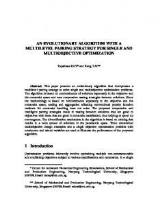
the performance of the improved PSO algorithm, this present paper tests six typical benchmark functions as in table I to compare DDPSO with SPSO. For the SPSO algorithm, traditional theory confirmed that the linear decline inertia weight works well for population search. Therefore, the interval ω ∈ [0.4,0.9] is chosen for the ω of the SPSO. For DDPSO algorithm, Jin [17] proved the SPSO a necessary condition ω ∈ [0.3333, 0.5] to convergence with mean square merit. In addition, the population size is set to 20 and the dimension of optimization functions is set to 2, the largest operation of each function is set to 1000 and the fault-tolerant iterations are 150. The other parameters will be set according to table II. In addition, table III shows the results about the average optimization and the variance of the optimization functions simulated by SPSO and DDPSO. Fig.1~Fig.6 represent the experimental simulations of the six typical benchmark optimization functions. According to the table III, we can see from Fig.1 and Fig.4 that both SPSO and DDPSO had good global search capability early in the evolution process. But DDPSO achieved better accuracy in less number of iterations by average than SPSO, and maintained high global and local search capabilities during the evolution process of the algorithm, so the result was better than the SPSO algorithm. Fig.2 showed that both of the two algorithms could converge to global optimization solution in a few iterations, but the DDPSO improved the average convergence rate. What can be drawn from Fig.3 and Fig.6 is that, in the later stage of evolution processes, DDPSO maintained high local search ability, and DDPSO achieved a higher convergence precision than SPSO. Fig.5 showed that, when dealing with function of Sphere’s f6, DDPSO maintains a higher global explore ability at the first, and achieved faster convergence rate than SPSO during the evolutionary processes.

TABLE I. TEST FUNCTIONS SELECTED FOR EXPERIMENT Name

Function 1 1 2 2 (x +y ) − n

1

Ackley

f1(x, y) = 20 + e−20e 5

Rastrigin

f 2 ( x) = ∑ [ xi2 − 10 cos(2π xi ) + 10]

− en

(cos(2π x)+cos(2π y))

Search Space

Optimal/position

(-30, 30)n

22.2956 (±29.5008, ±29.5008)

n

(-5.12, 5.12)n

Rosenbrock

f3 ( x ) =

n

∑ [100( x

i −1

− x i2 ) 2 + (1 − x i ) 2 ]

8 0 .7 0 6 6 ( ± 4 .5 2 , ± 4 .5 2 )

i

(-5.12, 5.12)n

0(1,…,1)

(-300, 300)n

0(0,…,0)

(-10, 10)n

0(0,…,0)

(-100, 100)n

0(0,…,0)

i

1 4000

n

∑ (x )

n ⎛ (x ) ⎞ +1 − Π cos ⎜ i ⎟ i =1 i⎠ ⎝

Griewank

f4 ( x) =

Schaffer's f6

f 5 ( x , y ) = 0 .5 +

Schaffer's f7

f 6 ( x, y ) = ∑ ( xi2 + yi2 )0.25 × [sin(50 × ( xi2 + yi2 )0.1 ) + 1.0]

i =1

i

2

(s in x i2 + y i2 ) 2 − 0 . 5 (1 + 0 . 0 1 ( x i2 + y i2 ) 2 ) 2

n

i =1



695

TABLE II. PERIMETERS SELECTION FOR DIFFERENT FUNCTIONS

ω

Functions

c1

c2

d1

d

2

∆x

Swarm Size

Ackley

[0.5 0.3333]

2

2

1.0e-003

5.0e-003

5.0e-006

20

Rastringin Rosenbrock

[0.5 0.3333] [0.5 0.3333]

2 2

2 2

1.0e-003 1.0e-003

1.0e-002 5.0e-003

1.0e-005 5.0e-006

20 20

Griewank

[0.5 0.3333]

2

2

1.0e-002

3.0e-003

1.0e-005

20

Shere’s f6

[0.5 0.3333]

2

2

1.0e-005

1.0e-003

1.0e-003

20

Shere’s f7

[0.5 0.3333]

2

2

1.0e-005

1.0e-004

1.0e-003

20

TABLE III. PERFORMANCE COMPARISON BETWEEN DDPSO AND SPSO Function

f1(x)

Dimension 2

PSO Average Optimization 22.23

Gmax 1000

Variance -6.5

DDPSO Average Optimization 22.2777

Variance -18.5

f 2 ( x)

2

1000

80.6975

5.1e-005

80.7055

f3 ( x)

2

1000

5.3e-013

-0.9e-026

3.7e-016

0.3e-007 1.4e-033

f 4 ( x)

2

1000

8.1e-003

0.2e-005

3.1e-013

1.2e-025

f 5 ( x)

2

1000

9.2e-017

2.8e-033

1.7e-016

1.7e-032

f 6 ( x)

2

1000

2.7e-013

1.8e-022

5.7e-015

1.2e-029

5

10 1.348

10

PSO 1.346

DDPSO

0

10

10

1.344

10

-5

gbest val.

gbest val.

10

1.342

10

-10

10 1.34

10

-15

10 1.338

10

PSO

DDPSO 1.336

-20

10

10

0

100

200

300 epoch

400

500

0

100

200

300

600

Figure 1. Trajectories of Ackley based on two algorithms.

400 epoch

500

600

700

800

Figure 3. Trajectories of Rosenbrock based on two algorithms. 2

10

0

10

1.9

10

-2

10

1.89

10

-4

10 1.88

gbest val.

gbest val.

10

1.87

10

-6

10

-8

10 1.86

10

-10

10 1.85

10

PSO

-12

10

DDPSO

PSO

1.84

10

DDPSO -14

10

0

50

100

150 epoch

200

250

Figure 2. Trajectories of Rastrigin based on two algorithms.


0

100

200

300 epoch

400

500

600

300

Figure 4. Trajectories of Griewank based on two algorithms.

696


0

the PSO algorithm, and the application background should also be considered. Second, the convergence rate or the time complexity of the modified algorithm needs to be estimated, and the following work will also analysis the sensitivity of the parameters when used in other typical complex optimization systems.

10

-2

PSO

10

DDPSO -4

10

-6

10

gbest val.

-8

10

-10

10

ACKNOWLEDGMENT

-12

10

-14

10

-16

10

-18

10

0

50

100

150

epoch

Figure 5. Trajectories of Sphere's f6 based on two algorithms.

This work was financially supported by the National Natural Science Foundation of China under Grant No.61064011. And it was also supported by China Postdoctoral Science Foundation, Science Foundation for The Excellent Youth Scholars of Lanzhou University of Technology, and Educational Commission of Gansu Province of China under Grant No.20100470088, 1014ZCX017 and 1014ZTC090, respectively.

2

10

0

REFERENCES

PSO

10

DDPSO -2

10

-4

10

gbest val.

-6

10

-8

10

-10

10

-12

10

-14

10

-16

10

0

20

40

60 epoch

80

100

120

Figure 6. Trajectories of Sphere's f7 based on two algorithms.

V. CONCLUTIONS A modified PSO with a decline disturbance index based on basic particle swarm optimization was presented in this paper. The modified algorithm effectively improved the deficiencies of the prone to local optimization solution and slow convergence by adding a decline disturbance index to the velocity updating formula of the evolutionary computing algorithm. Theoretical analysis, which is based on stochastic processes, proves that the trajectory of particle is a Markov processes and DDPSO algorithm converges to the global optimal solution with mean square merit. Experimental simulations show that the DDPSO algorithm has better performance on the convergence, and achieves better solutions in shorter time for typical benchmark functions than the standard PSO. Nevertheless, DDPSO also has some other problems to deal with compared with other original modified PSO algorithms. Thus, the further work needs to be done is as follows: First, On condition that the PSO algorithm converges with mean square merit, the range of parameters of the decline disturbance index should be determined to improve the convergence rate further of


[1] J. Kennedy and R. C. Eberhart, “Particle swarm optimization,” IEEE Symp. Neural Networks, vol. 4, pp. 1942-1948, December 1995, doi:10.1109/ICNN.1995.488968. [2] J. G. Jiang, Q. Wu and N. Xia, “Solving Agent coalition using adaptive particle swarm optimization algorithm,” CAAI Transactions on Intelligent Systems, vol. 2, pp. 6973, April 2007. [3] B. Luitel and G. K. Venayagamoorthy, “Quantum inspired PSO for the optimization of simultaneous recurrent neural networks as MIMO learning systems,” Neural Networks, vol. 23, pp583-586, June 2010, doi:10.1016/j.neunet.2009.12.009. [4] V. K. Patel and R. V. Rao, “Design optimization of shelland-tube heat exchanger using particle swarm optimization technique,” Applied Thermal Engineering, vol. 30, pp. 1417-1425, August 2010, doi:10.1016/j.applthermaleng.2010.03.001. [5] S. L. Ho, Shiyou. Yang, G. Z. Ni, E. W. C. Lo and H. C. Wong, “A particle swarm optimization–based method for multiobjective design optimizations,” IEEE Transactions on Magnetics, vol. 41, pp. 1756-1759, May 2005, doi:10.1109/TMAG.2005.846033. [6] H. Yoshida, K. Kawata, Y. Fukuyama and Y. Nakanishi, “A particle swarm optimization for reactive power and voltage control considering voltage security assessment,” IEEE Transactions on Power Systems, vol. 15, pp. 12321239, November 2000, doi:10.1109/59.898095. [7] F. Q. Zhao, Q. Y. Zhang, D. M. Yu, et al. “A hybrid algorithm based on PSO and simulated annealing and its applications for partner selection in virtual enterprise,” Lecture Notes in Computer Science, vol. 3644, pp. 380389, 2005, doi:10.1007/11538059_40. [8] S. L. Ho, S. Y. Yang, G. Z. Ni, E. W. C. Lo and H. C. Wong, “A Particle Swarm Optimization-Based Method for Multiobjective Design Optimizations,” IEEE Tansactions on Magnetics, vol. 41, pp. 1576-1579, May 2005, doi:10.1109/TMAG.2005.846033. [9] Y. Shi and R. Eberhart, “A modified particle swarm optimizer,” IEEE Int'1 Conf. Evolutionary Computation(ICEC 98), pp. 69-73, May 1998 doi:10.1109/ICEC.1998.699146. [10] F. Van de Berch and A. Engelbrech, “Cooperative learning in neural networks using particle swarm optimizers,” South African Computer Journal, vol. 26, pp. 84-90, 2000. [11] M. Clerc, “The swarm and the queen: towards a deterministic and adaptive particle swarm optimization,” IEEE. Evolutionary Computation(CEC 99), pp.1951-1957, 1999, doi:10.1109/CEC.1999.785513.


[12] Wang Hu and Z. S. Li, “A simpler and more effective particle swarm optimization algorithm,” Journal of Software, vol. 18, pp. 861-868, April 2007, doi:10.1360/jos180861. [13] Q. Y. He and Chuanjiu Han, “Improved particle swarm optimization algorithm with disturbance term,” Computer Science, vol. 4115, pp. 100-108, 2006, doi:10.1007/11816102_11. [14] D. B. Chen and C. X. Zhao, “Particle swarm optimization with adaptive population size and its application,” Applied Soft Computing, vol. 9, pp. 39-48, 2009, doi:10.1016/j.asoc.2008.03.001. [15] L. G. Tsoulos and A. Stavrakoudis, “Enhancing PSO methods for global optimization,” Applied Mathematics and Computation, vol. 216, pp. 2988-3001, 2010, doi:10.1016/j.amc.2010.04.011. [16] M. Clerc and J. Kennedy, “The particle swarm-explosion, stability, and convergence in a multidimensional complex space,” IEEE Transactions on Evolutionary Computation, vol. 6, pp. 58-73, February 2002, doi:10.1109/4235.985692. [17] X. L. Jin, L. H. Ma, T. J. Wu and J. X. Qian, “Convergence analysis of the particle swarm optimization based on stochastic processes,” ACTA AUTOMATICA SINICA, vol. 33, pp.1263-1268, March 2007, doi:10.1360/aas-007-1263.

Fuqing Zhao P.h.D., born in gansu, China, 1977, has got a P.h.D. in Dynamic Holonic Manufacturing System, Lanzhou University of Technology, gansu, 2006. He is a Post Doctor in Control Theory and Engineering in Xi’an Jiaotong University and Visiting Professor of Exeter University. His research work includes theory and application of pattern recognition, computational intelligence and its application, where more than twenty published articles index by SCI or EI can de found.


697

Fuqing Zhao, Yi Hong, Dongmei Yu, etal. A hybrid particle swarm optimisation algorithm and fuzzy logic for process planning and production scheduling integration in holonic manufacturing systems. International Journal of Computer Integrated Manufacturing 2010, SCI: 543WQ, EI:20100412670592 Fuqing Zhao, Yi Hong, Dongmei Yu, etal. A hybrid algorithm based on particle swarm optimization and simulated annealing to holon task allocation for holonic manufacturing system. The International Journal of Advanced Manufacturing Technology. 2007, SCI: 152KW Fuqing Zhao, Yahong Yang and Qiuyu Zhang. Timed PetriNet(TPN) Based Scheduling Holon and Its Solution with a Hybrid PSO-GA Based Evolutionary Algorithm(HPGA). Lecture Notes in Artificial Intelligence. 2006 SCI: IDS Number: BEY22, EI:064210172164

Jianxin Tang, born in Henan, China, 1985.12. His research interest is the theory and application of pattern recognition and artificial intelligence.

Jizhe Wang, born in Henan, China, 1986.8. His research work is the theory and application of pattern recognition and artificial intelligence.

Chunmiao Wei, born in Shanxi, China, 1984. His research interest is the application of pattern recognition, Graphics and Image Processing, Computer Vision.