AN IMPROVED REGIONAL ALGORITHM TO RETRIEVE TOTAL SUSPENDED PARTICULATE MATTER USING IRS-P4 OCM DATA a
Yaswant Pradhan a *, A. S. Rajawat a *, A. V. Thomaskutty a, M. Gupta a, C. R. C. Nagur b, Shailesh Nayak a * Marine & Water Resources Group, Space Applications Centre, ISRO, Ahmedabad 380 015, Gujarat, India * E-mail:
[email protected];
[email protected];
[email protected] b Institute of Marine Studies, University of Plymouth, Plymouth, Devon, PL4 8AA, UK
Commission VII KEYWORDS: SPM, Diffuse attenuation coefficient, Ocean colour, Radiometer, Case 2 water, Bay of Bengal
ABSTRACT: Data from six validation campaigns in the coastal waters of the Bay of Bengal (BOB) were used to develop a regional SPM (Suspended Particulate Matter) algorithm. The in situ data sets for this algorithm are composed of 60 stations with optical and 39 station with total SPM measurements, encompassing SPM concentrations between 13 and 189 mg L-1, with most of the observations in shallow (Case 2; average depth ~45 m) waters and a limited number of observations in Case 1 waters. A simple statistical analysis was carried out to evaluate the SPM concentration variation with diffuse attenuation coefficient, K(555) at 555 nm in the BOB coastal waters. The linear regression to the fit has coefficient of determination, r2 = 0.95 and a standard error of estimates σ = 15 mg L-1. The algorithm relating K(555) to Lwn(443)/Lwn(670) was also evaluated through regression analysis of radiometric profiles in the BOB. However, the new SPM algorithm failed to explain the estimates in Case 1 waters, where a spectral reflectance ratio algorithm [Tassan 1994] appears to produce better results. An integration of both the approaches performs better in generating the routine IRS-P4 OCM (Ocean Colour Monitor) SPM mapped product.
1. INTRODUCTION Accurate physical, biological and chemical measurements of the upper-ocean are essential for understanding the structures and processes that affect the climate and environment. Ocean colour observation with remote sensors from air and space platforms has become popular during the last decades because of its continuous coverage of the earth surface, which allows for the identification of zones characterised by physical and biological processes occuring at the sea surface. Ever since the launching of CZCS (Coastal Zone Color Scanner), mapping and quantitative estimation of the surface bio-geophysical constituents such as chlorophyll-a, suspended particulate material (SPM), and gelbstoff (coloured dissolved organic matter or CDOM), through the remote sensing of ocean colour has gone through a quiet revolution. Extensive studies were carried out to relate explicitly radiance/reflectance with in-water constituents in the past three decades [Morel and Prieur 1977, Gordon et al 1988, Sathyendranath et al 1994, Lee et al 1998, etc.]. Previous studies confirm that for Case 1 waters (devoid of direct influence of land runoff and littoral drift), most of the observed variations in the colour and transparency can be related to varying concentration of marine phytoplankton and their metabolism decay (CDOM). But the presence of highly variable contributions of suspended sediment and minerals by river discharge and the presence of exceptionally higher pigment and CDOM concentration makes the coastal (Case 2) waters more optically complex. Also the global colour ratio algorithms break down in Case 2 regime because of the presence of multiple substances, which do not co-vary with chlorophyll concentration. The Bay of Bengal is a region of large freshwater and sediment input [Emmel and Curray 1984], high sea-surface temperature,
and variable monsoonal forcing. The annual fresh water discharge into the bay exceeds 1.5 × 10¹² m3, which reduces the mean salinity by about 7‰ in the northernmost bay [Laviolette 1967]. The bay receives about 2 × 10⁹ tons of sediments annually, mostly contributed through the Himalayan Rivers - the Ganga and the Brahmaputra (G-B) from the north (figure 1); the Indian Peninsular Rivers - the Mahanadi, the Godavari, the Krishna etc. from the west; and the Irrawady and the Salveen from the east. It is, therefore, worth investigating the state of the surface particulate matters and their consequences over the bay, in the present context. The Ocean Colour Monitor (OCM) aboard IRS-P4 makes available the opportunity to estimate the concentrations of chlorophyll-a, SPM, gelbstoff at the sea surface and atmospheric aerosol in the marine environment. Originally, the SPM retrieval algorithm using OCM data followed a similar approach outlined by Tassan (1994), tuned in Indian waters, which is valid for lower SPM concentrations within 30% [Anonymous 2000]. To validate/modify this approach in coastal (Case 2) waters, SAC (Space Applications Centre) and GSI (Geological Survey of India) have conducted six campaigns in the coastal waters of the Bay of Bengal during 2000-2002. From these observations we found that, it makes sense to calibrate the ocean colour algorithms in terms of the diffuse attenuation coefficient, K (λ ) , in the Bay of Bengal coastal waters. Based on the in situ measurements, we could generalise that SPM concentrations are highly correlated with K(555), and propose a site-specific SPM algorithm with a standard error of estimates 15 mg L-1. Since most of the in situ observations were within the continental margin (average depth of ~45 m), we retain old (Tassan) approach valid for deeper waters (> 50 m depth) where we have very sparse measurements during the campaigns.
The International Archives of the Photogrammetry, Remote Sensing and Spatial Information Sciences, Vol. 34, Part VII
2. MEASUREMENTS AND MODEL DESCRIPTION The coastal cruise database (CCDB) is composed of six OCM validation campaigns (joint ISRO-GSI) in the Bay of Bengal during 2000-2002, onboard R. V. Samudra Kaustubh (ST-131, ST-136, ST-140, ST-142, ST-149, and ST-151). Measurements of total SPM, chlorophyll-a and optical parameters from over the continental margin (8.8 - 775 m with an average depth of ~45 m), off the east coast of India (80.20-88.65°E and 14.6-21.34°N), were drawn on to examine the variation in optical properties with SPM and chlorophyll concentrations. Over this region the sediment loads are very high (13 - 189 mg L-1), particularly at the head of the bay and at the river mouths. Since the pigment concentrations are very low (0.011 - 1.84 µg L-1, from CDDB), the changes in optical quantities are likely to be governed by inorganic sediments carried by major river systems in this region (figure 1), although the effects of pigment and CDOM are equally important in Case 2 waters.
basically deigned to collect photons travelling in specific directions (upward/downward), which can be converted into physical values (viz. spectral irradiance, radiance). LiCOR measures the upwelling irradiance, Eu ( z, λ ) and downwelling irradiance,
E d (z, λ ) within the wavelength domain 350 - 900 nm (continuous 1 nm interval). SPMR profiles both upwelling radiance, Lu ( z, λ ) and downwelling irradiance, E d (z, λ ) and SMSR measures the above surface incoming solar irradiance, E s (0+, λ ) , using DSP techniques and 24 bit A/D converters in 7 spectral channels [Satlantic User’s Manual 2000]. The optical sensor characteristics of Satlantic radiometer are akin of the Ocean Colour Monitor (OCM) [Anonymous 2000]. The apparent optical properties like, Water-leaving radiance, L w (λ ) , Remote Rrs (λ ) , Normalised water-leaving radiance, L wn (λ ) , and Diffuse attenuation coefficie nt, K (λ ) Sensing
Reflectance,
were computed (see appendix) as per standard protocols [Fargion and Mueller 2000]. The diffuse attenuation coefficient K(555) can be related to the ratio of normalised water-leaving radiance Lwn(443)/Lwn(670) as
Lwn (443) ln[K (555) − 0.07] = ln( A) + B ln Lwn (670)
(1)
where, A and B are the regression coefficients; and the attenuation coefficient for pure water, Kw(555) = 0.07 m-1, is the minimum possible value for K(555) [Jerlov 1976]. The calibrated single component algorithm for SPM in terms of diffuse attenuation coefficient, K(555) in coastal waters may be expressed as
SPM 2 = mK (555) + n
(2)
where, m and n, respectively, the slope and intercept of the linear regression. OCM TOA radiance Figure 1: Object of investigation – the Bay of Bengal coastal waters with major river systems and bottom topography (inset) 2.1 Suspended Particulate Matter: Suspended particulate materials (dry weight (mg L-1)) were determined gravimetrically as outlined in Strickland and Parsons (1972) and as specified in JGOFS protocols [UNESCO 1994]. Samples were filtered through 0.4 µm pre-weighed polycarbonate filters. The filters were washed with three 2.5 - 5 ml aliquots of distilled water and immediately dried in an oven at 75°C. The filters were then re-weighed in laboratory, using an electrobalance. 2.2 Radiometric measurements: Measurements of the underwater light field were performed with (i) LiCOR portable underwater spectro-radiometer, (ii) SeaWiFS Profiler Multi-channel Radiometer (SPMR), and (iii) SeaWiFS Multi-channel Surface Reference (SMSR). These instruments are
Atmospherically corrected (Landcloud masked) water-leaving radiance [1...6], Rrs [1…6], Lwn [1…6] (SAC Report 2000)
SPM 1 (Equation 7)
If SPM 1 > F1
K (555) from equation (1)
T
SPM 2 as in equation (2)
F
SPM = SPM 1∪ SPM 2 Figure 2: Schematic of the integrated model
The International Archives of the Photogrammetry, Remote Sensing and Spatial Information Sciences, Vol. 34, Part VII
The final product (SPM) is the integration of values below and above a case 1 flag, (F1 = 5.5 i.e. the boundary value at 50 m depth contour) from SPM1 [Tassan 1994] and SPM2 respectively. A schematic of the flow is shown in figure 2.
3. RESULTS AND DISCUSSION
The Case 1 SPM algorithm (SPM1) for OCM is a fine-tuning of Tassan’s approach in Indian waters [Anonymous 2000]:
SPM 1 =
Rrs(555) (7) 25 exp a0 + a1 ( Rrs(555) − Rrs(670) ) Rrs(490) where, 0 < SPM1 < 25 mg/L; a0 = 2.166; a1 = 0.991
In water diffuse attenuation coefficients can be calculated from in situ profiles of spectral irradiance and radiance field (see appendix). However, this is not possible from satellite measurements as it provides information at a single layer. Therefore, we propose an indirect method [similar as Austin and Petzold 1981] to estimate the in-water diffuse attenuation coefficients by establishing an empirical relationship with ratios of normalised water-leaving radiances, based on direct comparison with in situ radiometric profiles. Data from CDDB were combined to bring together a regression sample of size N = 59. The linear least-square fit to this data is
∗ lnK (555) − 0.07 =
Lwn (443) − 0.356251− 0.871654ln Lwn (670)
(3)
Figure 3(c) illustrates the scatter of in situ and modelled SPM. The maximum deviations from the regression fit occur at lower values of SPM. A comparison between SPM retrieved from OCM data with the new approach and using old algorithm (as in equation 7) is illustrated in figure 4. Plots of the resulting SPM distribution along two transects (figure 4 a) are shown in figure 5. There is a significant improvement in SPM concentrations as expected along the coastal waters and river mouths. 3.1
Validation match-ups:
CCDB data for ST 151 and few points from ST 131 cruise, which were not included in the calibration procedure, are being used to evaluate the performance of the new approach. Comparisons between OCM derived and in situ SPM are shown in Table 1. Table 1: Validation match-ups [OCM Vs in situ]
2
with coefficient of determination, r = 0.87, and a residual standard deviation of 0.226 (in log space).
Date ddmmyyyy
In situ SPM mg L-1 [hrs]
*OCM SPM mg L-1
13012000
27 [14:00]
05.789
15012000 03032002 03032002 04032002
20.2 [12:30] 14 [11:30] 15 [13:30] 12 [12:00]
27.391 12.572 13.973 10.579
04032002
12 [14:20]
11.594
05032002 05032002 07032002 07032002
13 [11:45] 11 [14:35] 12 [11:40] 10 [13:43]
18.153 09.012 16.344 15.853
Now equation (3) can be transformed as −0.87
∗ Lwn (443) K (555) = 0.07 + 0.7003 (4) Lwn (670) with a standard error of estimate, σ = 0.043 m-1, which is calculated as N ∗
∑ K (555) − K (555)
σ=
n =1
N −2
2
(5)
Water depth 775 m Water depth 22.89 m
March 03 OCM March 03 OCM Part. Cloudy Part. Cloudy Part. Cloudy Part. Cloudy
* OCM pass for all dates - 12:00 noon local standard time.
∗ where, K(555) is the model estimation and K (555) is from in situ profiles. Figure 3(b) illustrates the regression fit of the modelled K(555) and Lwn(443)/Lwn(670) (in log space). ∗ An empirical relationship between K (555) from irradiance profiles (see appendix) and measured in situ SPM is formulated, using equation (2), as: ∗
SPM 2 = 93.2 K (555) + 13. 24
Remarks
(6)
with a standard error of estimates 15 mg L-1, for 25 < SPM2 < 200 mg L-1. Scatter at different levels of SPM are shown in figure 3(a), where large discrepancies are observed at lower SPM concentrations.
4. OUTLOOK The initial results are encouraging; however, need more in situ observations, in both coastal and oceanic waters to evaluate the presumption in Case 1 waters. Measurements on the inherent optical properties (absorption and scattering) and other constituents (Chlorophyll, and Gelbstoff) are also proposed to fully understand the inter-relationship among various components and develop an analytical model rather than an empirical one.
The International Archives of the Photogrammetry, Remote Sensing and Spatial Information Sciences, Vol. 34, Part VII
N = 34 r = 0.97
100
(a) 50 0 0.0
0.5
1.0
1.5
2.0
mo delle d SPM, [mg/L]
150
1.5
model K(55 5), [/m]
S PM, [mg/L]
200
N = 83 rms = 0.043
1.0
(b)
0.5
0.0
1.0
K(5 55), [/m]
10.0
100.0
200
N = 34 r = 0.98
150 100
(c)
50 0
Lwn(443)/L wn(6 70)
0
50
100
150
200
in situ SPM, [mg/L]
Figure 3: Scattergram of in situ K(555) and SPM (a), Linear K(555) (modelled) versus a logarithmic scaling Lwn ratio (b), and modelled SPM versus in situ SPM (c)
Figure 4: Model outputs using IRS-P4 OCM data (17.33-22.18°N to 86.65-89.29°E): (a) SPM with integrated approach, (b) SPM with old algorithm, (c) K(555) as in equation (4) 1000.00
1000.00 100.00
Jan 13, 2000 Jan 15, 2000
10.00
SPM, [mg/L]
SPM, [mg/L]
100.00
1.00 0.10 0.01 0.00 86.00
10.00 1.00 0.10 0.01
87.00
88.00
89.00
Longitude, [°E]
90.00
0.00 16.00
18.00
20.00
22.00
24.00
Latitude, [°N]
Figure 5: Zonal (over 20.79°N; left panel) and meridional (over 87.89°E; right panel) variation of SPM (also depicted in fig. 4a) with old algorithm (thin lines) and new approach (thick lines).
References: Anonymous, 2000. Test & Evaluation Report on IRS-P4 OCM special product generation software, July 2000. IRS-P4/SAC/ RESA/MWRD/TR/12/2000, 29 pp. Austin, R. W., and Petzold, T. J., 1981. The determination of the Diffuse Attenuation Coefficient of Sea Water Using the Coastal Zone Color Scanner. Oceanography from Space (J. F. R. Gower Ed.), Plenum Press, New York, pp. 239-256. Chauhan, P., 2002. Personal Communication. Emmel, F. J., and Curray, J. R., 1984. The Bengal submarine fanNortheastern Indian Ocean. Geo-Mar. Lett. 3, pp. 199-124. Gordon, H. R., Brown, O. B., Evans, R. H., Brown, J. W., Smith, R. C., Baker, K. S., and Clark, D. K., 1988. A semi-analytic radiance model of ocean color. J. Geophys. Res., 93, pp. 10909 - 10924. Jerlov, N. G., 1976. Marine Optics. Elsevier, Amsterdam, 231 pp. Laviolette, P. E., 1967. Temperature, salinity and density of the World’s Seas: Bay of Bengal and Andaman Sea. Informal Rep. No. 67-57 (Naval Oceanographic Office, Washington DC. Lee, Z. P., Carder, K. L., Mobley, C. D., Steward, R. G., and Patch, J. S., 1998. Hyperspectral remote sensing for shallow waters. I. A semianalytical model. Appl. Opt., 37, pp. 6329 6338. Morel, A., and Prieur, L., 1977. Analysis of variations in ocean color. Limnol. Oceanogr., 22, pp. 709-722. Mueller, J. L., and Austin, R. W., 1995. Ocean Optics Protocols for SeaWiFS Validation, Revision 1. NASA Tech. Memo. 104566, Volume 25, S.B. Hooker, E.R. Firestone and J.G. Acker (eds.), NASA Goddard Space flight centre, Greenbelt, Maryland, 66 pp. Mueller, J. L., 2000. Ocean Optics Protocols for Satellite Ocean Color Sensor Validation, Revision 2. NASA Tech. Memo. 209966, Chapter 8 - 9, Giulietta S. Fargion and James L. Mueller (eds.), NASA Goddard Space flight centre, Greenbelt, Maryland, pp. 65-97. Neckel, H., and Labs, D., 1984. The solar radiation between 3,300 and 12,500 Å. Solar Physics, 90, pp. 205-258. Sathyendranath, S., Hoge, F. E., Platt, T., and Swift, R. N., 1994. Detection of phytoplankton pigments from ocean color: improved algorithms. Appl. Opt., 33, pp. 1081-1089. Satlantic user’s manual, 2000. SeawiFS Profiling Multichanel Radiometer User’s Manual SPMR/SMSR 041, Issue/Rev. 1/1, 44 pp. Strickland, J. D. H., and Parsons, T. R., 1972. A Practical Handbook of Seawater Analysis. Fisheries Research Board of Canada, 310 pp. Tassan, S., 1994. Local algorithms using SeaWiFS data for the retrieval of phytoplankton, pigments, suspended sediment, and yellow substance in coastal waters, Appl. Opt., 33, pp. 23692378. UNESCO, 1994. Protocols for Joint Global Ocean Carbon Flux Study (JGOFS) Core Measurements, Manuals and Guides. 29, 170 pp.
Acknowledgements: Authors are thankful to Dr. A. K. S. Gopalan, Director, SAC and Dr. R. R. Navalgund, Director NRSA, for their incessant encouragements and invaluable suggestions towards this work. Thanks are also due to the Dy. Director General, Marine Wing,
GSI, for facilitating R. V. Samudra Kaustubh for collecting the in situ measurements.
Appendix: In-water apparent light fields can be computed from the in situ radiance/irradiance profiles. The different apparent optical properties (AOP) are calculated as follows: 1.
Diffuse attenuation coefficient for downwelling irradiance:
K Ed ( z 0 , λ ) = −
1 ln E d [( z, λ )] dz ln [E d ( z0 , λ )]
where, z : water depth, λ : wavelength E d (z, λ ) may be substituted by Eu ( z, λ ) and Lu ( z, λ ) for the calculation of K E (λ ) and K L (λ ) respectively. u u 2.
Water-leaving radiance:
L w (λ ) =
1 − ρ (λ , ϑ ) 2 (λ ) ηw
Lu (0− , λ )
where, ρ is Fresnel reflectance (~ 0.021) at nadir angle ϑ
η w is the refractive index of seawater (~1.345) Lu (0−, λ ) is the upwelling radiance at null depth extrapolated from the profile
3.
Q-factor:
Qn (0 − , λ ) = 4.
Lu (0 − , λ )
Remote sensing reflectance:
Rrs (λ ) =
5.
E u (0 − , λ )
L w (λ )
E s (λ , 0+ )
Downwelling surface irradiance [equivalent E s (0+, λ ) ]:
E d (0+ , λ ) = (1 + α ) E d (0 − , λ )
where, α is Fresnel reflection albedo from air+sky (~0.043) E d (0−, λ ) is extrapolated from E d (z, λ ) profile 6.
Normalised water-leaving radiance:
L wn (λ ) = F0 (λ ) R rs (λ )
F0 (λ ) : extra-terrestrial solar irradiance 1984]
[Neckel and Labs