BNS Feature Scaling: An Improved Representation over TF·IDF for SVM Text Classification George Forman HP Laboratories HPL-2007-32R1 Keyword(s): Text classification, topic identification, machine learning, feature selection, Support Vector Machine, TF*IDF text representation. Abstract: In the realm of machine learning for text classification, TF·IDF is the most widely used representation for real-valued feature vectors. However, IDF is oblivious to the training class labels and naturally scales some features inappropriately. We replace IDF with Bi-Normal Separation (BNS), which has been previously found to be excellent at ranking words for feature selection filtering. Empirical evaluation on a benchmark of 237 binary text classification tasks shows substantially better accuracy and F-measure for a Support Vector Machine (SVM) by using BNS scaling. A wide variety of other feature representations were later tested and found inferior, as well as binary features with no scaling. Moreover, BNS scaling yielded better performance without feature selection, obviating the need for feature selection.
External Posting Date: August 6, 2008 [Fulltext] Approved for External Publication Internal Posting Date: August 6, 2008 [Fulltext] To be presented and published in ACM 17th Conference on Information and Knowledge Management. Napa Valley, CA, October 26-30, 2008
© Copyright ACM 17th Conference on Information and Knowledge Management 2008
BNS Feature Scaling: An Improved Representation over TF·IDF for SVM Text Classification George Forman Hewlett-Packard Labs Palo Alto, CA, USA
[email protected]
ABSTRACT In the realm of machine learning for text classification, TF·IDF is the most widely used representation for real-valued feature vectors. However, IDF is oblivious to the training class labels and naturally scales some features inappropriately. We replace IDF with Bi-Normal Separation (BNS), which has been previously found to be excellent at ranking words for feature selection filtering. Empirical evaluation on a benchmark of 237 binary text classification tasks shows substantially better accuracy and F-measure for a Support Vector Machine (SVM) by using BNS scaling. A wide variety of other feature representations were later tested and found inferior, as well as binary features with no scaling. Moreover, BNS scaling yielded better performance without feature selection, obviating the need for feature selection.
Categories and Subject Descriptors H.3.3 [Information Search & Retrieval]: Information filtering; I.5 [Pattern Recognition]: Design methodology, feature evaluation and selection.
General Terms Algorithms, Performance, Experimentation.
Keywords Text classification, topic identification, machine learning, feature selection, Support Vector Machine, TF*IDF text representation.
1. INTRODUCTION Text classification via machine learning is at the heart of effective document categorization, personalization, news filtering, and information routing. State-of-the-art classification accuracy can be achieved by applying a linear Support Vector Machine (SVM) to a ‘bag-of-words’ representation of the text, where each unique word in the training corpus becomes a separate feature [1][9][10]. The numerical feature value for a given word/term is often represented by its term frequency TF in the given text multiplied by its inverse document frequency (IDF) in the entire corpus—the ubiquitous ‘TF·IDF’ representation. IDF is commonly taken to be log( # documents ÷ # documents containing the term). By multiplying by IDF, the common functional words such as ‘of’ Permission to make digital or hard copies of all or part of this work for personal or classroom use is granted without fee provided that copies are not made or distributed for profit or commercial advantage and that copies bear this notice and the full citation on the first page. To copy otherwise, or republish, to post on servers or to redistribute to lists, requires prior specific permission and/or a fee. CIKM’08, October 26–30, 2008, Napa Valley California, USA. Copyright 2008 ACM 978-1-59593-991-3/08/10...$5.00.
and ‘can’ are devalued relative to the uncommon words that are more likely topic-specific indicators. Although TF·IDF is widely used in text classification, it is oblivious to the class labels in the training set, which can lead to inappropriate scaling for some features. Consider a toy example: a word X occurs in 80% of the positive training cases and another word Y occurs in only 3% of the positive cases—suppose neither occurs among the negative training cases. IDF gives a superlinear boost to words with lower frequency of occurrence. But in this case the more common word is a much stronger predictor. A specific, real example is illustrated later in Section 5.1. Filter methods for feature selection have developed a variety of metrics that do a good job of correctly ranking the predictive value of different features, e.g. Bi-Normal Separation (BNS) [4]. In this paper we improve on the state-of-the-art by using the BNS feature scoring metric in a new way: to scale the magnitude of the feature values. That is, we compute the BNS score for each feature and use TF·BNS for each feature value, replacing IDF. This increases the effect of important words on the kernel distance computations for the SVM. We show that this simple idea substantially improves SVM accuracy and F-measure on a benchmark of 237 binary text classification tasks, especially when TF is restricted to be binary. For comparison, we also tested a dozen other metrics and found that BNS scaling performed best. BNS feature selection was previously shown to substantially improve text classification [4]. One of the difficulties of feature selection, however, is in deciding the optimal number of features to use. The new method of BNS scaling offers to simplify the process, because it consistently performed best by using all features. This has an intuitive appeal of not ‘throwing away’ information. For those situations where the volume of data must be reduced for computational scalability at the cost of classification accuracy, we recommend a hybrid that uses Information Gain for feature selection and BNS for feature scaling, based on our empirical study.
1.1 Related Work and Scope In this space of classification research, some work addresses binary classification [4][9][13], as in information filtering, e.g. separating spam from good email. Other work addresses multiclass classification [17], e.g. routing or classifying a document into one of many categories. Our focus here is on binary classification, but we expect the results to generalize. Binary tasks are an important sub-problem in most multi-class classification methods, which decompose the 1-of-n problem by pitting each class against the others. Finally, we note that the problem n-of-m multi-class classification, e.g. topic recognition, is addressed by m independent binary classifiers.
may be different than the metric used for feature scaling. The best method found by our experiments is such a hybrid: IG used for feature selection and BNS for feature scaling.
There is a large research literature in feature selection metrics to filter words for text classification. The goal is often to improve accuracy, but in some papers it is to preserve accuracy as much as possible as the number of features is reduced in order to decrease computational workload. In this work our goal is simply to maximize classification performance, as measured by accuracy and F-measure. However, in the process, we developed a method that satisfies both goals.
2.3 Feature Scoring Metrics The primary feature scoring metrics we use in this paper are defined as follows.
As a side note, in non-text domains, there has been a lot of work that takes a collection of features with widely disparate ranges and normalizes or discretizes them to make them palatable for induction algorithms. These concerns led to the common practice of normalizing the feature space for SVMs. Instead, we modify the normalization phase as an additional opportunity to condition the data for learning. Finally, there are many references to ‘feature scaling’ or ‘feature weighting’ in the literature that simply refer to variations on normalization. For example, word counts are sometimes scaled so that long documents appear to have a uniform number of words as short documents. In contrast, this work scales the feature ranges based on the supervised labels. The closest references to this sort of feature weighting in the literature are in lazy learning (case-based learning), where the goal is to learn an appropriate distance function so that the nearest neighbors of a novel case suggest appropriate class labels [15]. Such methods constitute iterative wrapper searches to adjust the feature weights of a (linear) distance metric. By contrast, in our work, we let the SVM perform the inductive learning, and we simply condition the input feature vectors with a single, fast pass over the training set. Any of the feature scoring metrics and IDF can be computed in a single linear scan the training corpus.
Bi-Normal Separation (BNS):
| F-1(tpr) – F-1(fpr) |
Inverse Document Freq (IDF):
log( (pos+neg) ÷ (tp+fp) )
Log Odds Ratio [13]:
log( (tp·tn) ÷ (fp·fn) )
Information Gain (IG):
H(data) – H(data | word)
= H(pos,neg) – (P(word) H(tp,fp) + (1-P(word)) H(fn,tn) ) where pos = number of positive training cases, typically minority, neg = number of negative training cases, tp = number of positive training cases containing word, fp = number of negative training cases containing word, fn = pos – tp, tn = neg – fp, true positive rate tpr=P(word | positive class) = tp/pos, false positive rate fpr=P(word | negative class) = fp/neg, P(word) = (tp+fp) / (pos+neg), entropy H(x,y) = –nln(x/(x+y)) – nln(y/(x+y)), nln(x) = x log2 x, and F-1 is the inverse Normal cumulative distribution function, as commonly available from statistical tables. Note that these are computed using binary word features, i.e. many occurrences of a word in a single document only count toward one tp or fp count. Information Gain and BNS are naturally symmetric with respect to positively and negatively correlated features. Log Odds Ratio, however, assigns a very low score to a strongly predictive feature that occurs in almost all negative cases but in none of the positive cases. To rectify this, for any negatively correlated features we reverse the meaning of a word occurrence to be a word non-occurrence, i.e. tp ↔ fn and fp ↔ tn. This solution improves a number of feature selection metrics that otherwise ignore strong negative features [4].
2. METHODS Here we briefly define the feature scoring metrics and how they are used for feature selection and/or for feature scaling.
2.1 Feature Selection via Filtering Filtering methods for feature selection evaluate each feature independently via a chosen scoring metric. Then, some number of top-scoring features is selected for input to the induction algorithm. One can either specify the number of top-ranked features to select, or equivalently, specify a particular score threshold, which is particular to the feature scoring metric being used. In order to compare different scoring metrics on a common x-axis scale, the former is often preferable in research.
As usual, there are some nuances to converting these straightforward mathematical definitions to robust code. For example, Log Odds Ratio is undefined if tp, tn, fp, or fn is zero. To avoid this, we substitute 0.5 for any zero count, which has the desirable property that even if some of the variables are zero, the function remains responsive to the magnitude of the other variables. Likewise, for IG we define nln(x) = 0, whenever x = 0. Finally, in the BNS function, the inverse Normal goes to infinity at zero or one; hence, we limit tpr and fpr to the range [0.0005, 1-0.0005]. Laplace smoothing is a more common method to avoid these extreme probabilities, but it damages the maximum likelihood estimate, and it loses the good performance of BNS by devaluing many valuable negative features in favor of very rare positive features [4]. Alternately and perhaps preferably, one could substitute a fractional count if tp or fp is exactly zero; this may work better for extremely large training sets. We used a fixed limit because we used a finite size lookup table for the inverse Normal function, generated by Gnuplot’s invnorm() function and transferred to our Java code, since this standard statistical function is not available in the Java math libraries.
2.2 Feature Scaling The key idea of this paper is to use a feature scoring metric to make the numeric range greater for more predictive features, just as IDF attempts to do in TF·IDF. This affects the dot-product distance between cases as evaluated by the linear SVM kernel [9]. For example, if the BNS score is 2.1 for the word feature ‘free’ in a spam classification task, then its Boolean presence or absence in a document would be represented as either 0 or 2.1, rather than 0 or 1. A less predictive word ‘cat’ with a BNS score of 0.3 would have the smaller range 0 or 0.3, and therefore have less effect on the kernel distance computations. This basic idea can be applied to any scoring metric. Furthermore, it can also be applied to nonbinary features, e.g. to scale term frequency TF counts: TF·BNS. Additionally, feature scaling may be used in conjunction with feature selection. The scoring metric used for feature selection
2
F-measure requires the classifier have good precision and good recall on the positive class, whereas good accuracy can be achieved simply by predicting all test cases as negative, if the positive class is rare.
3. EXPERIMENT DESIGN Our experiments consider a wide variety of text feature representations. For each potential feature scoring metric, we consider using it as a scale factor on TF feature counts and separately as a scale factor on binary features. We also consider plain binary features, as well as raw, unscaled TF features. In Section 4.6, we also combine scaling with feature selection.
For each of the 237 binary text classification tasks, the performance of the learning algorithm is measured via standard 4-fold stratified cross-validation, repeated with eight different random split seeds (kept consistent for each representation tested). Note that all feature selection and scaling is determined from only the training folds within cross-validation, to avoid leaking information from the test set.
3.1 Benchmark Datasets The benchmark text classification tasks we use are drawn from Reuters-21578 (re), OHSUMED abstracts (oh), the Los Angeles Times (la), the Foreign Broadcast Information Service (fbis), the Web ACE project (wap), and various TREC competitions (tr, new3), originally compiled by Han and Karypis [7]. See Table 1, which includes the total vocabulary size and the average number of words present per document. There are 19 multi-class datasets and their class sizes vary widely. For these experiments we consider each class vs. all others within that dataset, yielding 237 binary text classification tasks, which are representative of the size and difficulty of many of the industrial text classification tasks we face at HP Labs.
For any given feature representation under study, we obtain 237 x 8 performance measurements. To distill these into one summary number, we use macro-averaging, weighting each of the measurements equally (as opposed to micro-averaging, which would weight them according to the number of documents that happen be available in each task).
3.3 Induction Algorithms We use the linear SVM implementation provided by the WEKA library v3.4 [16]. In this experiment, we use its default behavior, rather than attempting to optimize each of its many parameters. In particular, its default complexity constant is one. We had to disable its feature space normalization feature, otherwise it rescales all feature values to the range [0,1]. Thus, BNS feature scaling causes the more important features to have a greater effect on the SVM kernel dot product than less predictive features.
Although the tasks are not entirely independent of each other because of some overlap in their negative classes, they are much more independent than studies that consider only a single source of documents with a common negative class, e.g. using just Reuters. We have made the processed TF feature vectors available for other researchers at the WEKA web site [16]. Table 1. Benchmark text classification datasets Dataset fbis la1 la2 new3 oh0 oh10 oh15 oh5 ohscal re0 re1 tr11 tr12 tr21 tr23 tr31 tr41 tr45 wap
Classes 17 6 6 44 10 10 10 10 10 13 25 9 8 6 6 7 10 10 20
Docs 2463 3204 3075 9558 1003 918 1050 913 11162 1504 1657 414 313 336 204 927 878 690 1560
Words 2000 31472 31472 26833 3182 3012 3238 3100 11465 2886 3758 6429 5804 7902 5832 10128 7454 8261 8460
This kernel-centric explanation of the effect is specific to kernelbased classifiers such as the SVM, but we found that the BNS scaling also helps some other classification models that are not based on kernels. We repeated the experiment protocol with the multinomial Naïve Bayes classifier, which has been shown superior to its simple binomial form for text classification [11]. (Note that feature scaling would have no effect on the classic binomial formulation, which converts each feature to binary nominal values. The multinomial formulation uses word counts, which BNS scaling effectively increases for the more important features.) We found that while BNS scaling does benefit the multinomial Naïve Bayes classifier, its best performance came from using plain binary features with BNS feature selection, and even then it had substantially worse accuracy than SVM— consistent with much of the literature. Thus, we report the Naïve Bayes results only in a tech report [2]. Henceforth we just consider SVM models.
Words/Doc 160 151 148 235 53 56 59 54 60 52 53 282 274 470 385 269 195 281 141
4. EMPIRICAL RESULTS Initially we focus on the BNS feature scoring metric (the initial impetus for this work) and contrast it with IDF or no scaling, since they are most common. Later in Section 4.5 we compare against many other feature scoring metrics that we considered later.
3.2 Evaluation Measures
4.1 Accuracy & F-measure
We evaluate performance based on two standard performance measures: accuracy for its historical standard in machine learning research and F-measure for its improved sensitivity in the common information retrieval situation where positives are rare. F-measure is the harmonic average of precision & recall, where precision = true positives ÷ predicted positives, and recall = true positives ÷ all positives in ground truth. To achieve good
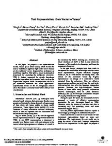
Figure 1 shows the average accuracy and F-measure for six different text representations, including error bars which extend above and below each point by one standard error, stdev÷sqrt(N). Binary features and term frequency (TF) counts are considered for each of three feature scaling methods: IDF, BNS, and no scaling. The two most common text representations, TF·IDF and binary features, both performed significantly worse than BNS scaling of
3
0.80
BNS
TF.BNS
binary
TF.IDF
IDF
TF
0.75
0.70
BNS
TF.BNS
binary
TF
IDF
97
TF.IDF
Accuracy
F-measure
98
Figure 1. SVM accuracy (left) and F-measure (right) for six different text feature representations, including standard error bars. axis ranges are identical to make it clear that the SVM precision typically exceeded its recall.
binary features (labeled just ‘BNS’). We expected this from the intuitive motivation in the introduction. BNS scaling leverages the class labels to improve the distance evaluations of the SVM kernel. Using binary features, as opposed to term frequencies, consistently improves accuracy; binary features do not appear to have a consistent effect on F-measure, but we elucidate this next. Overall, the BNS-scaled binary features provided a 1% improvement over TF·IDF for accuracy and 7% for F-measure, both with no question of statistical significance by their small error bars in proportion to the differences.
Here we can see consistent effects. Using binary features yields a large improvement in precision compared with TF features. Likewise, BNS scaling results in a large improvement in recall compared with IDF or no scaling. (We will explain the underlying cause of this in the discussion section, as well as the additional data point labeled ‘hBNS.’) Together, these two effects make for a substantial increase in F-measure. The dotted curved lines in the background show points of equal F-measure, indicating the gradient to obtain better F-measure performance.
4.2 Precision vs. Recall Analysis
Since the positive class is typically small for text classification, the best improvement in accuracy is by improving precision, not recall—hence, the consistent benefit of binary features on accuracy we observed in Figure 1. (Note: for applications where the best precision is sought regardless of recall, one may prefer instead to optimize the precision in the top N predicted positives.)
Good F-measure requires a balance between precision and recall. It can be informative to see the tradeoffs these different methods make between precision and recall at the classifier’s natural classification threshold. (Alternately, one could consider full precision-recall curves by sweeping through all decision thresholds, but this considers many decision points for which the classification algorithm was not attempting to optimize and makes it difficult to compare six methods.) Figure 2 shows Precision vs. Recall for the six methods considered in the previous figure, including standard error bars in both dimensions. The x- and y-
4.3 The Effect of Class Distribution The importance of BNS scaling increases as the class distribution becomes more skewed. To illustrate this, we have binned together those benchmark tasks that have between 0% and 5% positive cases, 5%—10% positives, and so forth. See Figure 3, which shows macro-average F-measure for each bin and again includes standard error bars. When the minority class is relatively
0.90 binary
BNS hBNS
IDF
0.80
TF.BNS 0.90
F-measure
Precision
0.95
TF TF.IDF
0.85 0.80 0.75
0.70
BNS binary IDF
0.70 0.65
0.70
0.80
0.90
0
Recall
5
10
15
20
25
% positives
Figure 2. Precision & Recall for six text representations. The thin dotted lines show isoclines of equal F-measure.
Figure 3. The benefit of BNS feature scaling grows as the percentage of positive cases becomes small. 4
0.95
TF counts
0.90 BNS
F-measure
0.85
TF.BNS binary
0.80
TF IDF
0.75
TF.IDF
0.70
wap tr11 re1 ohsca fbis oh10 re0 oh15 tr31 tr21 la1s tr12 la2s oh5 new3s oh0 tr23 tr45 tr41
0.65
BNS Log Odds Ratio Log Chi Squared Odds Ratio Chi Squared no scaling F-measure of word Balanced Accuracy (tpr–fpr) IDF Pointwise Mutual Information Log Probability Ratio Pearson Correlation Prob. Ratio (tp/pos ÷ fp/neg) Accuracy of word (tp–fp) Information Gain 0.50 0.55
Figure 4. BNS feature scaling typically dominated other methods for the 19 datasets. balanced (20%–25%), the benefit of BNS scaling vs. no scaling or IDF scaling of binary features is small. As the percentage of positives decreases to a small minority, the classification performance naturally drops for all methods, but the decline is substantially less if BNS scaling is used. In other words, the benefit of BNS scaling is greater for highly imbalanced classification problems. Each successive bin contains roughly half as many benchmark tasks, indicating that the performance under high skew is the more common operating range for text classification problems.
binary features (sort key)
0.60 0.65
0.70 0.75
0.80 0.85
F-measure
Figure 5. F-measure for 30 different text representations. benchmark problems as independent). Many of the methods, including IDF, performed worse than using no scaling. We note that the runner up was Log Odds Ratio. (We included its formula in Section 2.3, partly because it is extremely easy for researchers and practitioners to adopt in their code, whereas BNS requires statistical tables not available in common software libraries.) Our prior study showed that Odds Ratio has a preference surface that is similar to BNS. For feature selection, the dynamic range of the scoring metric is immaterial—only the relative ranking of features is important. But here, we find that the logarithm of Odds Ratio did a better job of conditioning the feature vectors for the linear SVM kernel than using raw Odds Ratio, which has a very large range. Similarly for Chi-Squared and Probability Ratio.1
4.4 Per-Dataset Views Next we show the macro-average F-measure for each of the 19 datasets separately. Although the graph is cluttered, Figure 4 shows clearly the near-complete dominance of BNS scaling of binary features (labeled ‘BNS’). To aid the visualization, we have sorted the classes by their BNS performance. BNS did not dominate for three of the most difficult datasets, where instead TF·BNS performed best. Note that the performance of some of the methods can be quite erratic, e.g. for datasets tr21 and tr23 the methods IDF and binary performed extraordinarily poorly.
4.6 Feature Selection & Scaling Combined Finally, we consider the question of whether performance might further be improved by its use in conjunction with feature selection, since feature selection has been shown beneficial, esp. with BNS and IG [4]. In Figure 6 we vary the number of features selected, with and without BNS scaling on binary features (all performance figures were worse for TF features, so they are not shown in order to reduce visual clutter). The rightmost point on the logarithmic x-axis is not to scale, but indicates that all features were used within each dataset, i.e. no feature selection. The overall best performance for both accuracy and F-measure is obtained using BNS scaling with all features. Without BNS scaling, the best available performance is obtained by selecting a subset of features via BNS. (The lack of improvement with IG feature selection and certain other methods has led some researchers in the past to conclude that SVM does not benefit from feature selection.)
4.5 Comparing Many Other Scoring Metrics At first, we tested the feature scaling idea with only the BNS metric and the Information Gain metric, because these two were the leaders for feature selection in our prior study [4]. But this begs the question of whether some other feature scoring metric might perform yet better. To resolve this question, we tested all the feature selection metrics of our prior study, where their many formulae can be found. Note that asymmetric functions, such as the Probability Ratio [13], have been adjusted to symmetrically value strong features that happen to be correlated with word absence rather than word presence. To these we added Pearson Correlation and Pointwise Mutual Information [10]. Altogether, fifteen choices for feature scaling (all supervised except for IDF and ‘no scaling’) are paired both with TF counts and separately with binary features in Figure 5. Although some future metric may be devised that exceeds BNS, the present evidence indicates that BNS with binary features is statistically significantly better— it passes a paired two-tailed t-test against the runner-up with p