taken into account by means of a custom kernel design. In ..... app. Fig. 2. Classification in the PLP and acoustic waveform do- mains for all phoneme classes ...
CUSTOM-DESIGNED SVM KERNELS FOR IMPROVED ROBUSTNESS OF PHONEME CLASSIFICATION Jibran Yousafzai1 , Zoran Cvetkovi´c1 , Peter Sollich2 Department of Electronic Engineering1 and Department of Mathematics2 , King’s College London, WC2R 2LS, UK
ABSTRACT The robustness of phoneme classification to additive white Gaussian noise in the acoustic waveform domain is investigated using support vector machines. We focus on the problem of designing kernels which are tuned to the physical properties of speech. For comparison, results are reported for the PLP representation of speech using standard kernels. We show that major improvements can be achieved by incorporating the properties of speech into kernels. Furthermore, the high-dimensional acoustic waveforms exhibit more robust behavior to additive noise. Finally, we investigate a combination of the PLP and acoustic waveform representations which attains better classification than either of the individual representations over a range of noise levels. Index Terms— Kernels, Phoneme classification, Robustness, Support vector machines, PLP 1. INTRODUCTION Automatic speech recognition (ASR) systems lack the level of robustness inherent to human speech recognition (HSR) [1]. In recognizing syllables or isolated words, the human auditory systems performs above chance level already at −18dB SNR and significantly above it at −9dB SNR [2]. No ASR system is able to achieve performance close to that of human auditory systems under severe noise.While language and context modelling are essential for reducing many errors in speech recognition, accurate classification of isolated phonetic units is very important for achieving robust recognition of continuous speech. Most of the state-of-the-art ASR front-ends are some variant of MFCC, RASTA or PLP [3]. These representations are derived from the short term magnitude spectra followed by non-linear transformations to model the processing of the human auditory system. They remove variations from speech signals that are considered unnecessary for recognition while preserving the information content. Therefore, they have a much lower dimension than acoustic waveforms, and this facilitates the estimation of probability distributions. However it is not certain that in the process of “peeling off” speech components that are unnecessary for recognition, one is not discarding some of the information that makes speech such a robust message representation. To make these state-of-theart representations of speech robust to noise, several methods have been proposed to reduce explicitly the effect of noise on spectral representations [4] in order to approach the optimal performance which is achieved when the training and test-
ing conditions are matched [5]. Our recent study on phoneme classification [6] with support vector machines (SVMs) shows that although classification in the PLP domain exhibits superior performance when the test phonemes are corrupted by low levels of noise, classifiers in the high-dimensional acoustic waveform domain trained in quiet conditions with straightforward noise adaptation are more robust in severe noise. PLP is designed in a way which removes non-lexical invariances (sign, time alignment), however for recognition in the acoustic waveform domain these invariances need to be taken into account by means of a custom kernel design. In this paper, we focus on the design of SVM kernel functions for acoustic waveforms of speech. Classification in the PLP representation domain using standard SVM kernels is also reported. Applying the method of [6], we show further that a convex combination of the decision functions of the PLP and acoustic waveform SVM classifiers results in a superior performance across a wide range of SNRs. Our experiments demonstrate the effectiveness of custom designed kernels for robust phoneme classification under adverse conditions. It should be emphasized that this study is focused on phoneme classification for comparison of the acoustic waveform and PLP representations of speech although we believe the results also have implications for the construction of continuous speech recognition systems. The SVM approach to classification of phonemes is presented in Section 2. Custom-designed kernels for the classification task in the acoustic waveform domain are described in Section 3. Section 4 presents techniques for noise adaptation in both the PLP and acoustic waveform domains. The classification results in the PLP and acoustic waveform domains detailing the effects of kernels on the accuracy are reported in Section 5, where we also discuss the combination of the PLP and acoustic waveform representations for improved accuracy. Finally, Section 6 draws some conclusions. 2. CLASSIFICATION METHOD An SVM [7] estimates decision surfaces separating two classes of data. In the simplest case these are linear but for speech recognition, one typically requires nonlinear decision boundaries. These are constructed using kernels instead of dot products, implicitly mapping data points to high-dimensional feature vectors. A kernel-based decision function which classifies an input vector x is expressed as h(x) = ∑ αi yi hϕ (x), ϕ (xi )i + b = ∑ αi yi K(x, xi ) + b i
i
(1)
where ϕ is a non-linear mapping function while xi , yi = ±1 and αi , respectively, are the i-th training sample, its class label and its Lagrange multiplier. K is a kernel function and b is the classifier bias determined by the training algorithm. Two commonly used kernels are the polynomial and radial basis function (RBF) kernels given by (2) and (3), respectively, Kp (x, xi ) = (1 + hx, xi i)Θ ,
(2)
80
40
CLEAN − /aa/
40
20
20 0 0 80
1
2
3
4
0 0 40
NOISY − /aa/
1
2
3
4
2
3
4
3
4
NOISY − /v/
60 40
2
Kr (x, xi ) = e−Γkx−xi k . (3) To obtain a multiclass classifier, binary SVM classifiers are combined via error-correcting code methods [8]. A standard approach is to use K(K − 1)/2 pairwise classifiers, each trained to distinguish two of the K classes. For a test point x, we then predict the class k for which dk (x) = ∑Kl=1,l6=k ξ (hkl (x)) is minimized, where ξ is some loss function and hkl (x) is the output of the classifier trained to distinguish classes k and l, with sign chosen so that a positive sign indicates class k. We compared a number of loss functions ξ (h); the hinge loss ξ (h) = max(1 − h, 0) performed best and is used throughout this paper.
CLEAN − /v/
60
20
20 0 0
1
2
3
4
0 0
1
80 ADAPTED − /aa/ 60
40 ADAPTED − /v/
40
20
20 0 0
1
2
3
4
0 0
1
2
3. CUSTOM-DESIGNED KERNELS
Fig. 1. Histograms of log-energies of phoneme classes /aa/ and /v/ for clean waveforms, noisy waveforms at 0dB SNR adapted waveforms as specified in (8) i.e. and noise 2 2 log kxk − σ
The most important issue in any SVM classification task is the use of appropriate kernels that express prior knowledge about the physical properties of the data sets. To this end, for classification using acoustic waveforms, we use an even kernel (Ke ) [6] to account for the fact that a speech waveform and its inverted version are perceived as being the same. An even version of a kernel K can be obtained as
Since PLP, MFCC and other state-of-the-art representations are based on short-time magnitude spectra and so also contain information on the energy, using similar customdesigned kernels for classification in the PLP domain will not have any advantage over the standard (polynomial or RBF) kernels and this was confirmed in our experiments.
Ke (x, xi ) = K(x, xi ) + K(x, −xi ) + K(−x, xi ) + K(−x, −xi ) . (4) Here K(x, xi ) can by any kernel that satisfies Mercer’s theorem. In this paper, we use the polynomial kernel, Kp for both PLP and waveform representations. However, evaluating Kp for acoustic waveforms requires normalization of x and xi to give a sensible estimate of their closeness i.e. Kp (x, xi ) = (1 + hx/ kxk , xi / kxi ki)Θ . This is used as a baseline kernel for the acoustic waveform representations whereas Kp defined in (2) is used for the PLP representations. A further invariance of acoustic waveforms, to time alignment, can be incorporated into Ke by defining a shift-invariant even kernel (Ks ) of the form Ks (x, xi ) =
n 1 ∑ Ke (xu∆ , xiv∆ ) , (2n + 1)2 u,v=−n
(5)
where ∆ is the shift increment, [−n∆, n∆] is the shift range, and xu∆ is a segment of the same length as the original waveform x0 but extracted from a position shifted by u∆ samples. The log-energy distributions of waveforms of phoneme classes /aa/ and /v/ are shown in Figure 1 (top). By comparing the distributions of energy of these phoneme classes, we observe that the energy of isolated phoneme segments can be very useful in distinguishing them. Therefore, we embed this information into the kernel and define a norm-dependent shift-invariant even kernel (Kn ), 2
Kn (x, xi ) = e−(logkxk
2
−logkxi k2 ) /2a2
Ks (x, xi ) ,
(6)
4. NOISE ADAPTATION To improve the performance in both domains, we perform noise adaptation of the features extracted from our test data. Since the noise variance, σ 2 can be estimated during pause intervals (non-speech activity) between speech signals, we assume that its value is known. For the PLP representations, the features are standardized, i.e. scaled and shifted to have zero mean and unit variance on the training set. As mentioned previously, the optimal performance with PLP is obtained under matched training and test conditions [5]. However, this is an impractical target which could be achieved only if one had access to a large set of classifiers trained for different noise types and levels. Therefore, in order to have a fair comparison of PLP with acoustic waveforms, we use classifiers trained in quiet conditions and adapt them to noise using cepstral mean and variance normalization (CMVN) [4], a noise compensation technique that modifies the cepstral coefficients in order to minimize the mismatch between the training and test data. Here, training is performed on PLP features standardized in quiet conditions, but in testing features are scaled and shifted so as to standardize them on the training set corrupted with a noise level matching the test conditions. The training set is used here rather than a small development set to get the best possible estimate of noise cepstral mean and variance. By attempting to ’decouple’ the speech information from the noise information, CMVN can significantly improve the performance of PLP classifiers. It should be noted that in practice, cepstral mean and variance are estimated from a limited
Kp (x, xi ) = (1 + hx, ˜ x˜i i)Θ ,
(7)
while Ke and Ks are as defined in (4) and (5) respectively. Similar adaptation as in the polynomial kernel is also required in the norm-dependent kernel (6). Figure 1 shows the distribution of log-energies of phoneme classes /aa/ and /v/ and motivated incorporating the energy information into the kernel. However, the energy distributions of noisy waveforms changes significantly as illustrated in Figure 1 (middle) for an SNR of 0dB. Under the assumption that speech and noise are uncorrelated, subtraction of the estimated noise variance (σ 2 ) from the energy of the noisy phoneme should result in distributions of the energies that are very similar to those of the clean waveforms and this is indeed the case for our data (Figure 1, bottom). We, therefore, use this subtracted energy in evaluating the norm-dependent kernel (6), giving 2
Kn (x, xi ) = e−(log|kxk
2
−σ 2 |−logkxi k2 ) /2a2
Ks (x, xi ) ,
(8)
As training for acoustic waveforms is performed in quiet conditions, noise adaption of the training data xi is not required. The absolute value of the subtracted energy is used to catch the rare cases when speech and noise are anti-correlated. In the next section, we compare the performance of these kernels with standard SVM kernels for the phoneme classification task in the acoustic waveform domain. Furthermore, classification results in the PLP domain are used as benchmarks for comparison with acoustic waveforms. 5. EXPERIMENTAL SETUP Experiments are performed on the TIMIT database [11]. Training and testing is done on the ’si’ and ’sx’ sentences of TIMIT. The training set consists of 3696 sentences from 168 different speakers. The core set is used for testing which consists of 192 sentences from 24 different speakers not included in the training set. We remove the glottal stops /q/ from the labels and fold certain allophones into their corresponding phonemes using the standard Kai-Fu Lee clustering [12]. This results in a total of 48 phoneme classes. Furthermore, among these 48 phoneme classes, there are 7 groups for which the contribution of within-group confusions towards
100
90
80
ERROR [%]
data set rather than the entire corrupted training set and hence would not be as accurate. Therefore, one would expect the practical results for PLP to be worse compared to the ones presented here. However, we use them as a benchmark for comparison with acoustic waveforms. Another common approach to reduce the mismatch between training and test data is the multi-condition/multi-style training of PLP classifiers [9]; however, CMVN and its variants generally perform better [10]. In the case √ of acoustic waveforms, the test data is normalized to 1 + σ 2 whereas the training data is set to have a unit norm for computation of the inner product in the polynomial kernel. This is done to keep the norm of the speech signal roughly independent of the noise. Explicitly, √ let x˜ = x 1 + σ 2 /kxk and x˜i = xi /kxi k for a test waveform x and training waveform xi . Then the kernel for the normalized waveforms are
70
60
PLP: K (CMVN) p PLP: Kp (Matched) Waveform: K p Waveform: Ke Waveform: Ks Waveform: K n Combined:λapp
50
40
30
−18
−12
−6
0 6 SNR [dB]
12
18
Q
Fig. 2. Classification in the PLP and acoustic waveform domains for all phoneme classes except silence (/sil/, /cl/, /vcl/, /epi/). Different kernels are used for the classification of acoustic waveforms and the results are compared with PLP.
multiclass error is not counted [12]: (/sh/, /zh/), (/aa/, /ao/), (/ah/, /ax/), (/el/, /l/), (/en/, /n/), (/ih/, /ix/), (/sil/, /cl/, /vcl/, /epi/). As silence forms a major portion of TIMIT, we first isolate the problem of discriminating speech and silence. This is achieved by training a top-level one-vs-rest classifier to discriminate between silence (/sil/, /cl/, /vcl/, /epi/) and the rest of the 44 phoneme classes. In order to then discriminate between these 44 non-silence classes, 946 one-vs-one classifiers are trained and combined via error correcting code methods for multiclass classification. Regarding the binary SVM classifiers, comparable performance is obtained with polynomial and RBF kernels for the PLP representation so we show results for the former. For the waveform representation, results are reported for different custom-designed kernels; as expected Kn (8) performed best. Fixed hyperparameter values are used throughout for training binary SVMs: the degree of the polynomial kernel, Θ = 6 and the penalty parameter C = 1. For the acoustic waveform representation, phoneme segments are extracted from the TIMIT sentences by applying a 76.5 ms rectangular window at the center of each phoneme waveform (of variable length), which at 16 kHz sampling frequency gives fixed length vectors in R1224 . In the evaluation of Ks defined in (5), we use a shift increment of ∆ = 50 samples (≈ 3 ms) over a shift range ±100 (so that n = 2), giving five shifted segments of length 1024 samples each. In evaluating Kn , two values for a are selected, (0.5, ∞). The decision function values corresponding to each value of a are added together to give the final score. For the PLP representation, we convert each waveform into a sequence of 13 dimensional feature vectors. Then, the 6 frames (75 ms duration) closest to the center of a particular phoneme are concatenated to give a representation in R78 . Since the calculation of time derivatives and second order derivatives of the PLP features uses information about several adjacent frames, they are not used in our experiments in order to have a fair comparison with
100 PLP: K (CMVN) p PLP: K (Matched) p Waveform: Kn Combined:λ
90
1
0.8
app
80
0.6
λ
ERROR [%]
70 60
0.4
50
0.2 40
0
30 −18
−12
−6
0 6 SNR [dB]
12
18
Q
Fig. 3. Classification in the PLP and acoustic waveform domains for all phoneme classes including silence. A top-level one-vs-rest classifier is trained to discriminate between silence and all the rest of the phoneme classes.
acoustic waveforms. In this study, we focus on investigating robustness in the presence of additive white Gaussian noise. To test the classification performance of PLP and acoustic waveforms in noise, we normalize each sentence to unit energy per sample and then add a noise sequence with variance σ 2 (per sample) to the entire sentence. It should be noted that SNR at the sentence level is thus fixed but SNR at the level of individual phonemes will vary widely. Classification results using SVMs in the PLP and acoustic waveform domains are shown in Figure 2 and 3. In Figure 2, results are reported for the task of classification among all phoneme classes except silence. For acoustic waveforms, classification results with different kernels are presented. As explained above, polynomial kernel is used for classification of PLP features. One observes that a PLP classifier trained on clean data gives very good performance when tested on clean data. (The actual error rate of 32% is somewhat higher than in previous work [13] due to the exclusion of the silence class and the derivative information from cepstral features as explained above.) But at 0dB SNR, we get an error of 77% even with CMVN. In practice, these results would deteriorate even more as explained in Section 4. This can now be contrasted with the results for a classifier based on acoustic waveform data. One observes that the polynomial kernel performs worse than PLP for all SNRs. Incorporating sign-invariance of acoustic waveforms into the kernel gives an average improvement of around 5%. The largest improvement, by 7% is achieved at 12dB SNR. Adding shiftinvariance to the kernel improves the results even further. In quiet conditions, an 8% improvement is achieved over the even-polynomial kernel and the results are consistently better for all SNRs. Finally, we observe that adding to the kernel noise-adapted energy information about the phoneme segments improves the results especially in high noise e.g. a further 5% improvement over Ks is achieved at −6dB SNR.
−18
−12
−6
0 6 SNR [dB]
12
18
Q
Fig. 4. Optimal and approx. values of λ for a range of test SNRs. λ = 0 corresponds to PLP classification with CMVN, λ = 1 corresponds to waveform classification. By comparing the classification results for PLP with acoustic waveforms, we observe that the PLP classifiers give excellent performance at low noise. However the waveform classifiers exhibit a more robust behavior to noise and achieve improvments over PLP for noise levels above a crossover point between 12dB and 18dB SNR. In Figure 3, we report results for all phoneme classes including the silence class. The best results for both domains are compared here: polynomial kernel for PLP, and Kn for acoustic waveforms. We observe a similar behavior as seen previously. The PLP classifiers perform extremely well in low noise conditions with an error rate of e.g. 27% in quiet but perform poorly in high noise. For instance, 80% error is observed for PLP at −6dB SNR. The acoustic waveform classifiers do not perform as well in quiet conditions but exhibit a robust behavior to noise e.g. at −6dB SNR, an improvement of 12% is achieved over PLP. The crossover point beyond which waveforms perform better is again between 12dB and 18dB SNR. It should be emphasized that best performance using acoustic waveform classifiers is obtained when training is performed on clean data; training on noisy data (results not shown) leads to poorer performance. Next, we apply the method of [6] to combine classifiers based on waveforms and PLP. We will see that this attains better classification performance than either of the individual representations. We consider a convex combination of the decision values of the classifiers in the individual feature spaces. For classifiers h p (x) and hw (x) in the PLP and waveform domains respectively, we define the combined classifier output as � � (9) hc (x) = λ (σ 2 )hw (x) + 1 − λ (σ 2 ) h p (x) . Here λ (σ 2 ) is parameter which needs to be selected, depending on the noise variance, to achieve optimal performance. These binary classifiers are then combined for multiclass classification as described previously. The top-level one-vs-all binary classifiers for the PLP and acoustic waveform representations are combined in a similar manner for discriminating
silence from all the other phoneme classes. In Figure 4, the “optimal” λ (σ 2 ) i.e. the values of λ (σ 2 ) which give the minimum classification error for a given SNR of the test phoneme, are shown marked by ’o’. The error bars give a range of values of λ (σ 2 ) for which the classification error is less than the minimum error (%) + 2%. An approximation of the optimal λ (σ 2 ) is also shown in Figure 4 (solid line) and given by
λapp (σ 2 ) = α +
β �, 1 + σ02 /σ 2
(10)
with α = 0.2, β = 0.6 and σ02 = 0.03. In Figure 3, we compare the classification performance in the feature space of PLP and acoustic waveforms with the combined classifier for λapp (σ 2 ) selected according to (10). One observes that the combined classifier often performs better or at least as well as the individual classifiers. Furthermore, we found no significant difference in the performance of the combined classifier for the optimal λ (σ 2 ) and the approximation λapp (σ 2 ). Moreover, the values of optimal λ (σ 2 ) for different SNRs suggest that the combination of the PLP and acoustic waveforms is not simply acting as a switch between the two representations. The convex combination of the PLP and waveforms, in fact, helps to reduce the error in noise as shown in the Figure 3. Although the combined classifier does not achieve the impractical target of PLP classifier trained and tested in matched conditions, the gain in the classification accuracy is significant compared to a standalone PLP classifier with CMVN. A similar behavior of the combined classifier with λapp (σ 2 ) selected according to (10) can be observed for the task of phoneme classification without the silence class as shown in Figure 2. 6. CONCLUSIONS The robustness of phoneme classification to additive white Gaussian noise in the PLP and acoustic waveform domains was investigated using SVMs. We observe that embedding invariances and information that is necessary for recognition into the kernel can significantly improve the classification performance. While PLP representation allows very accurate classification of phonemes especially for clean data, its performance suffers severe degradation at high noise level. On the other hand, the high-dimensional acoustic waveform representation, although not as accurate as PLP classification on clean data, is more robust in severe noise. Our results further demonstrate that a convex combination of classifiers can achieve performance that is consistently better than for both individual domains for a wide range of SNRs. We are currently working on the phoneme classification task using multi-layered, multi-class SVMs [14, 15] with preliminary experiments giving encouraging results. In future work, we plan to investigate methods to embed information from adjacent frames/phonemes into the kernel for improved robustness. This would be done in order to be consistent with the time derivatives and second order derivatives of the PLP features.
7. REFERENCES [1] J. Sroka and L. Braida, “Human and Machine Consonant Recognition,” Speech Comm., 2005. [2] G. Miller and P. Nicely, “An Analysis of Perceptual Confusions among some English Consonants,” J. of the Acous. Soc. of America, vol. 27, no. 2, pp. 338–352, 1955. [3] H. Hermansky, “Perceptual Linear Predictive (PLP) Analysis of Speech ,” J. of the Acous. Soc. of America, vol. 87, pp. 1738–1752, Apr. 1990. [4] O. Viikki and K. Laurila, “Cepstral domain segmental feature vector normalization for noise robust speech recognition,” Speech Comm., vol. 25, pp. 133–147, 1998. [5] M. Gales and S. Young, “Robust continuous speech recognition using parallel model combination,” IEEE Trans. on Speech and Audio Processing, pp. 352–359, Sept. 1996. [6] J. Yousafzai, Z. Cvetkovi´c, P. Sollich, and B. Yu, “Combined PLP-Acoustic waveform classification for robust phoneme recognition using support vector machines,” EUSIPCO 2008, Aug. 2008. [7] V. N. Vapnik, The Nature of Statistical Learning Theory, Springer-Verlag, New York, 1995. [8] T. Dietterich and G. Bakiri, “Solving multiclass learning problems via error-correcting output codes,” J. of AI Research, vol. 2, pp. 263–286, 1995. [9] M. Holmberg, D. Gelbart, and W. Hemmert, “Automatic speech recognition with an adaptation model motivated by auditory processing,” IEEE Trans. on Audio, Sp. & Lang. Proc., vol. 14, no. 1, pp. 43–49, 2006. [10] J. Droppo, L. Deng, and A. Acero, “Evaluation of the splice algorithm on the aurora2 database,” EuroSpeech, 2001. [11] W. Fisher, G. Doddington, and K. Goudie-Marshall, “DARPA Speech Recognition Research Database,” DARPA Sp. Recogn. Workshop, pp. 93–99, 1986. [12] K. F. Lee and H. W. Hon, “Speaker-independent phone recognition using hidden markov models,” IEEE Trans. Ac. Speech Sig. Proc., vol. 37, no. 11, 1989. [13] P. Clarkson and P. J. Moreno, “On the use of support vector machines for phonetic classification,” ICASSP, 1999. [14] K. Crammer and Y. Singer, “On the algorithmic implementation of multiclass kernel-based vector machines,” J. Mach. Learn. Res., vol. 2, pp. 265–292, 2002. [15] K. Crammer and Y. Singer, “On the learnability and design of output codes for multiclass problems,” Machine Learning, vol. 47, no. 2-3, pp. 201–233, 2002.