Uncertainties in geotechnical engineering design are unavoidable. These uncertainties and ... the evaluation of the probability of failure pf (equation 1) different methods like Monte ..... Reliability and statistics in geotechnical engineering.
Budelmann, Holst & Proske: Proceedings of the 9th International Probabilistic Workshop, Braunschweig 2011
Response surface method in advanced reliability based design Maximilian Huber, Bernhard Westrich Pieter A. Vermeer, Christian Moormann Institute of Geotechnical Engineering, University of Stuttgart, Germany
Abstract: A design method is defined as a method to make decision under uncertainties encountered in a structural design process. In geotechnical engineering, the EUROCODE [1, 2] offers reliability techniques to take the uncertainty into account. Within this contribution the COLLOCATION BASED STOCHASTIC RESPONSE SURFACE METHOD as an alternative approach to the well known FIRST ORDER RELIABILITY METHOD is presented and applied in two parametric studies.
1
Introduction
Uncertainties in geotechnical engineering design are unavoidable. These uncertainties and associated risks can be quantified to improve design in geotechnical engineering. This is recognized in a recent National Research Council (2006) report on Geological and Geotechnical Engineering in the New Millennium: Opportunities for Research and Technological Innovation. The report remarked that “paradigms for dealing with … uncertainty are poorly understood and even more poorly practiced” and advocated a need for “improved methods for assessing the potential impacts of these uncertainties on engineering decisions …” [22]. In order to understand the consequences of uncertainty in geotechnical engineering, efficient methods to quantify the impact of soil variability and parameter uncertainty are needed. This contribution focuses on two reliability methods, which can be used within the reliability based design framework: the well known FIRST-ORDER-RELIABILITY METHOD (FORM) is compared to a new approach, called COLLOCATION STOCHASTIC BASED RESPONSE SURFACE METHOD (CSRSM). In addition to the theoretical background, two parametric studies are presented, in which the two methods are compared.
1
Huber, Westrich, Vermeer & Moormann: Response surface method in advance reliability based design
2
Uncertainty analysis in geotechnical engineering
The presence of uncertainties and their significance as related to design has long been appreciated. The engineer recognizes, explicitly or otherwise, that there is always a chance of not achieving the design objective. This element of risk arises, in part, from the inability to assess loads and resistances with absolute precision. Traditionally, the engineer relies primarily on empirical factors of safety to reduce the risk of adverse performance (collapse, excessive deformations, etc.) to an acceptable level. However, the relationship between the factor of safety and the underlying probability of failure is not a simple one. A larger factor of safety does not necessarily imply smaller probability of failure, because its effect can be negated by the presence of larger uncertainties in design. In addition, the effect of the factor of safety on the underlying probability of failure is also dependent on how conservative the design models and the design parameters are. As stated by PHOON [26]; the problem associated with the traditional method of ensuring safety can be resolved by rendering broad, general concepts, such as uncertainty and risk, into precise mathematical terms that can be operated upon consistently. This approach essentially forms the basis of reliability based design (RBD), in which uncertain engineering quantities (e.g. loads, capacities) are remodelled by random variables. A general scheme for uncertainty analysis in RBD is shown by DE ROCQUIGNY [14] in Figure 1. In the first step the mechanical model of the system is set up together with criteria for design and assessment of this structure. In a next step, the quantification of sources of uncertainty is done by the introduction of random variables. Via this, different uncertainties for e.g. material properties, geometry or loading can be taken into account, which is the basis for the uncertainty propagation. Herein, the response of the system is modelled and evaluated in terms of the probability of failure. The final step is the sensitivity analysis of the system, in order to quantify the contribution of the random variables to the system response as shown in [14, 27, 35]. The Authors refer to SUDRET [33], who presents among others in detail different methods for the classification of uncertainty, propagation methods to evaluate the response variability, the reliability and the sensitivity of a model.
Figure 1. General sketch for uncertainty analysis [14].
2
Budelmann, Holst & Proske: Proceedings of the 9th International Probabilistic Workshop, Braunschweig 2011
2.1
Response surface method
A vast number of literatures offer various techniques to evaluate the reliability of a system, which is captured via limit state equation. The limit state equation describes the performance of a system. In this context, the evaluation of the probability of failure pf is defined as the occurrence of a negative limit state function describing the collapse of the system. For the evaluation of the probability of failure pf (equation 1) different methods like Monte Carlo Simulation, First-Order-Reliability-Method (FORM), Importance Sampling, Directional Sampling, Subset Simulation or Line Sampling can be used among others according to BUCHER [12].
)
(
pf = Prob ⎡⎢g X1,X 2 ,....X n ≤ 0⎤⎥ = ∫ ... ⎣ ⎦
2.2
∫
g(X)≤0
f (x) dx X
(1)
First-Order-Reliability Method
FORM aims at using a first-order approximation of the limit-state function in the Gaussian space at the so-called most probable point (MPP) of failure pf (or design point), which is the limit-state surface closest point to the origin (Figure 2). Finding the coordinates of the MPP consist in solving a constrained optimization problem [11]. In addition to the coordinates of the MPP, also the influencing factors αc’ and αϕ’ can be evaluated via FORM, which describe the contribution of the random variable to the probability of failure. This can be interpreted also in a graphical way, as shown in Figure 2. The reliability index β represents the distance from the origin to the design points in the Gaussian space. The firstorder approximation of the failure probability is then given by pf = Φ(−β), where Φ is the standard normal cumulative distribution function [12]. Gaussian space ξϕ’ αϕ’ β
ξc’ αc’
μϕ’ tan
(c’*|ϕ’*) g0
nt ge
friction angle ϕ’ [°]
physical space
g>0 g 0 with Ii = ⎨ ⎪⎩α i ≠ j = 0
(11)
Parametric studies
The application of both approaches to two parametric studies is presented in this section. Two different kind of limit state equations were chosen to show the different features of the presented approaches: On the one hand side, a known limit state equation for the evaluation of the stability of a tunnel face is presented. Moreover, a nonlinear FEM program is used for the evaluation of the limit state equation of the serviceability of a strip footing on a layered soil.
3.1
Tunnel face stability
3.1.1
Deterministic problem
During construction of shallow tunnels using earth pressure balanced machines, the face stability is an important issue. To minimize settlements at the ground surface and to prevent an uncontrolled collapse of the soil, a necessary support pressure must be calculated. This estimation of the required support pressures for e.g. earth pressure balance (EPB) shields to ensure the stability of the face has been a topic of research until the present day [5, 19, 20, 24, 30, 32, 37]. LECA & DORMIEUX [20] present an upper bound solution for the face stability of shallow tunnels by using a kinematic approach. This upper bound solution involves three solutions based on consideration of three mechanisms, which are derived from the motion of rigid conical blocks. They identified three collapse mechanisms including two active and one passive mechanism. The passive blow-out mode of failure does not occur for the cases currently encountered in practice, as reported by MOLLON ET AL. [24]. Therefore this collapse mechanism is not investigated within this contribution. The concept of the limit state design has been picked up by ANAGNOSTOU & KOVÀRI [5] later. Recently SOUBRA [32] and MOLLON ET AL. [24] presented elaborations on this limit state design. VERMEER ET AL. [37] as well as RUSE [30] followed a different approach in evaluating the stability of a tunnel heading. Herein, no assumptions on the shape of the collapse mechanism are made. By using Finite Element Method (FEM) a formula was derived for the failure pressure pcollapse of the tunnel face (equation 12). For this purpose a 3D FEM program was used to model the stability of a tunnel heading under drained conditions using the Mohr-Coulomb failure criteria. Herein c’ is the effective cohesion, ϕ’ the effective friction angel, γ the unit weight of the soil and D the diameter of the circular tunnel (Figure 3). Is the ratio of overburden and diameter of the tunnel D bigger than H / D ≥ 1.5, the overburden and the load q at the surface have no influence onto the failure pressure pcollapse as well as on stiffness, dilatation angel and Poisson’s ratio of the soil [37].
7
Huber, Westrich, Vermeer & Moormann: Response surface method in advance reliability based design
⎛
⎞ 1 − 0.05 ⎟⎟ ⎝ 9 ⋅ tan ϕ ' ⎠
pcollapse = − c′ ⋅ cot ϕ ' + γ' ⋅ D ⋅ ⎜⎜
(12)
g = p / pcollapse – 1
(13)
3.1.2
Reliability analysis and sensitivity using FORM and CSRSM
The deterministic and stochastic soil properties in Table 1 were used to evaluate the reliability of the system. For this purpose the software package FERUM [11] was used for the evaluation of the probability of failure pf for the different levels of the face pressure p. The results of this study are shown in the Figure 4. Generally speaking, it can be deduced that the higher the face pressure, the higher the reliability of the system. FORM and CSRSM represent this qualitatively in the same way. The influence of the cohesion c’ and of the friction angle φ’ remains constant while varying the face pressure p. To enlighten the concept of CSRSM, the collocation points for different PCE orders are plotted in the Gaussian as well in the physical space (Figure 6). The dependency of the statistical moments to the PCE order is shown in Figure 5. Together with the results of Figure 7 and Figure 8, the reader can see the convergence of the CSRSM approximation. The mean value, the variance, the skewness and also the kurtosis show only minor changes at the PCE order M = 5. This can also be deduced from Figure 7: The PCE order M = 5 is acceptable for the probability of failure pf .This is strengthened the graphs of the empirical error and the coefficient of determination in Figure 5. The difference of both approaches can be clearly seen in Figure 4. The lower the probability of failure, the bigger is the difference of FORM and CSRSM. This is due to the approximation of the system response via a PCE within CSRSM, which becomes more inaccurate with deceasing probability of failure. The difference between the two approaches is not that striking while looking at the sensitivity of the cohesion and the friction angel in Figure 4. The dependency of the Sobol indices to the PCE order M is rather low, which is enlightened in Figure 9. q γ’, c’, ϕ’
H D
p
Figure 3. Geometry of the tunnel (left) and incremental displacement at failure of a tunnel face (right) presented in RUSE [30].
8
Budelmann, Holst & Proske: Proceedings of the 9th International Probabilistic Workshop, Braunschweig 2011
Table 1. Soil properties of the parametric study on the tunnel face stability. c’ = 2.5 kN/m² ϕ’ = 35 °
COVc’ = 20 % COVϕ’ = 10 %
lognormally distributed lognormally distributed
γ’ = 18 kN/m³
deterministic
D = 10 m p = 0 – 160 kN/m²
deterministic deterministic
Figure 4. Comparison of CRSRM and FORM in terms of the probability of failure, the reliability index and the sensitivity of the cohesion and the friction angel. -5
1 coefficient of determinitation
empirical error
2
x 10
1.5 1 0.5 0
2
4 PCE order M
6
0.9998 0.9996 0.9994
2
4 PCE order M
6
Figure 5. Accuracy of the CRSRM described by the empirical error and the coefficient of determination.
9
Huber, Westrich, Vermeer & Moormann: Response surface method in advance reliability based design
Figure 6. Collocation points in Gaussian space and physical space for several PCE orders.
10
2
0.4
1.5
0.3
Variance
Mean value
Budelmann, Holst & Proske: Proceedings of the 9th International Probabilistic Workshop, Braunschweig 2011
1
0.1
0.5 0
0.2
1
2
3 4 PCE order M
5
0
6
0.8 0.6 0.4
3 4 PCE order M
5
6
2
3 4 PCE order M
5
6
1.5 1 0.5
0.2 0 1
2
2
Kurtosis
Skewness
1
1
2
3 4 PCE order M
5
6
0
1
Figure 7. Statistical moments of the approximated system response for a face pressure p = 40 kN/m². -2
proability of failure pf
10
-4
10
-6
10
-8
10
0
2 4 PCE order M
6
Figure 8. Probability of failure for different orders M of the PCE.
Figure 9. Sobol indices for several orders of the PCE for a face pressure p = 40 kN/m².
11
Huber, Westrich, Vermeer & Moormann: Response surface method in advance reliability based design
3.2
Serviceability of a strip footing
3.2.1
Deterministic problem
To enlighten the above described approaches, another parametric study was carried out. For this reason, the settlement behaviour of a strip footing on a stochastic soil layer is investigated as shown in Figure 10, which follows the work of several authors [6, 28, 33, 35]. The Finite Element software PLAXIS [4] was used to evaluate the limit state equation (14). Herein, the settlements of the strip footing due to a load of p = 200 kN/m² are compared to a threshold dult = 0.50 m. The behaviour of the soil was modelled by the linear elastic, ideal plastic constitutive model using a non structured mesh with 15 noded elements. g = d – dult
(14)
Table 2 shows the stochastic and deterministic soil properties of both layers together with the properties of the deterministic geometry. 3.2.2
Reliability analysis and sensitivity using FORM and CSRSM
Figure 11 sows the probability of failure versus the coefficient of variation (COV) of the modulus of elasticity (EA, EB). It is obvious that the probability of failure increases with increasing variability. The differences between the two approaches are small. Focusing on the accuracy of the CSRSM, it can be deduced from Figure 12 that the PCE order M = 4 is sufficient for this problem. The results of the sensitivity evaluation are shown in Figure 11. Again, a similar result of the FORM and CSRSM can be observed. The influencing factors αi as well as the Sobol indices δi show the same influence: the higher the variability of the modulus of elasticity, the higher is the influence of the stiffness of the upper layer. In Table 3, the number of calls of the limit state equation is listed for different COV and for different PCE orders. It can be seen that FORM converged in a fast way in this simple problem. The benefit of the CSRSM would be more obvious, if a change of the dult would be investigated: In this case, the whole FORM algorithm would have to be started again. Within CSRSM, this can be done in the post-processing within a small amount of computational time compared to FORM. Moreover, CSRSM has not the convergence problems like FORM. But on the other hand, CSRSM cannot be recommended for the reliability problems with probability of failure smaller than pf 10-6. It can be concluded, that FORM and CSRSM can be used for the reliability and sensitivity analysis of complex system. The focus of future research will cover the incorporation of random fields to represent spatisal variability. Moreover, adaptive algorithms will be used to cover also the evaluation of small probabilities of failure.
14
Budelmann, Holst & Proske: Proceedings of the 9th International Probabilistic Workshop, Braunschweig 2011
5
References
[1] CEN (2002): Eurocode: Basis of structural design. European standard, EN 1990: 2002, April 2002. [2] CEN (2004): Eurocode 7 Geotechnical design - Part 1: General rules. EN 19971:2004, November 2004, European Committee for Standardization: Brussels, November 2004. [3] M. Abramovich and I.A. Stegun. Handbook of Mathematical Functions with Formulas, Graphs and Mathematical Tables. Dover, 1974. [4] R. Al-Khoury, K.J. Bakker, P.G. Bonnier, H.J. Burd, G. Soltys, and P.A. Vermeer. PLAXIS 2D Version 9. R.B.J. Brinkgreve and W. Broere and Waterman, 2008. [5] G. Anagnostou and K. Kovari. Face stability conditions with earth-pressure-balanced shields. Tunnelling and Underground Space Technology, 11(2):165–173, 1996. [6] G.B. Baecher and J.T. Christian. Reliability and statistics in geotechnical engineering. John Wiley & Sons Inc, 2003. [7] M. Berveiller, B. Sudret, and M. Lemaire. Presentation of two methods for computing the response coefficients in stochastic finite element analysis. In Proc. 9th ASCE specialty Conference on Probabilistic Mechanics and Structural Reliability, Albuquerque, USA, 2004. [8] M. Berveiller, B. Sudret, and M. Lemaire. Stochastic finite element: a non intrusive approach by regression. Revue Européenne de Mécanique Numérique-Volume, 15(12):81–92, 2006. [9] G. Blatman. Adaptive sparse polynomial chaos expansions for uncertainty propagation and sensitivity analysis. PhD thesis, Université Blaise Pascal, Clermont-Ferrand, 2009. [10] G. Blatman and B. Sudret. An adaptive algorithm to build up sparse polynomial chaos expansions for stochastic finite element analysis. Probabilistic Engineering Mechanics, 25(2):183–197, 2010. [11] J.-M. Bourinet, C. Mattrand, and V. Dubourg. A review of recent features and improvements added to ferum software. In Proc. of the 10th International Conference on Structural Safety and Reliability (ICOSSAR’09), Osaka, Japan, 2009. [12] C. Bucher. Computational analysis of randomness in structural mechanics. CRC Press, 2009. [13] C. Bucher and T. Most. A comparison of approximate response functions in structural reliability analysis. Probabilistic Engineering Mechanics, 23(2-3):154–163, 2008. 15
Huber, Westrich, Vermeer & Moormann: Response surface method in advance reliability based design
[14] E. De Rocquigny, N. Devictor, and S. Tarantola, editors. Uncertainty in industrial practice. Wiley Online Library, 2008. [15] A. Dutfoy, I. Dutka-Malen, A. Pasanisi, R. Lebrun, F. Mangeant, J. Sen Gupta, M. Pendola, and T. Yalamas. OpenTURNS, an Open Source initiative to Treat Uncertainties, Risks’N Statistics in a structured industrial approach. 41emes Journees de Statistique, SFdS, Bordeaux, Bordeaux, France, 2009. [16] A.I.J. Forrester, A. Sobester, and A.J. Keane. Engineering design via surrogate modelling: a practical guide, volume 226. Wiley, 2008. [17] S. Huang, S. Mahadevan, and R. Rebba. Collocation-based stochastic finite element analysis for random field problems. Probabilistic engineering mechanics, 22(2):194– 205, 2007. [18] S.S. Isukapalli. Uncertainty analysis of transport-transformation models. PhD thesis, Rutgers, The State University of New Jersey, 1999. [19] A. Kirsch. On the face stability of shallow tunnels in sand. PhD thesis, Universität Innsbruck, 2009. [20] E. Leca and L. Dormieux. Upper and lower bound solutions for the face stability of shallow circular tunnels in frictional material. Geotechnique, 40(4):581–606, 1990. [21] M. Lemaire and M. Pendola. PHIMECA-SOFT. Structural safety, 28(1-2):130–149, 2006. [22] A.C.S. Long, B. Amadei, J.-P. Bardet, J. T. Christian, S. D. Glaser, D. J. Goodings, E. Kavazanjian, D. W. Major, J. K. Mitchell, M.M. Poulton, and J. C. Santamarina. Geological and Geotechnical Engineering in the New Millennium: Opportunities for Research and Technological Innovation. The National Academies Press, 2006. [23] P. Malliavin. Stochastic analysis, volume 313. Springer Verlag, 1997. [24] G. Mollon, D. Dias, and A.H. Soubra. Face stability analysis of circular tunnels driven by a pressurized Shield. Journal of Geotechnical and Geoenvironmental Engineering, 136:215–229, 2010. [25] G. Mollon, D. Dias, and A.H. Soubra. Probabilistic analysis of pressurized tunnels against face stability using collocation-based stochastic response surface method. Journal of Geotechnical and Geoenvironmental Engineering, 137:385–395, 2011. [26] K.K. Phoon. Reliability-based design of foundations for transmission line structures. PhD thesis, Cornell University, 1995. [27] K.K. Phoon, editor. Reliability-based design in geotechnical engineering: computations and applications. Taylor & Francis, 2008.
16
Budelmann, Holst & Proske: Proceedings of the 9th International Probabilistic Workshop, Braunschweig 2011
[28] R. Popescu, G. Deodatis, and A. Nobahar. Effects of random heterogeneity of soil properties on bearing capacity. Probabilistic engineering mechanics, 20(4):324–341, 2005. [29] R. Rackwitz. Response surfaces in structural reliability. Technical Report 67, Laboratorium für den konstruktiven Ingenieurbau, Technische Universität München, 1982. [30] N.M. Ruse. Räumliche Betrachtung der Standsicherheit der Ortsbrust beim Tunnelvortrieb. PhD thesis, Institute of Geotechnical Engineering, University of Stuttgart, 2004. [31] A. Saltelli. Sensitivity analysis in practice: a guide to assessing scientific models. John Wiley & Sons Inc, 2004. [32] A.H. Soubra. Kinematical approach to the face stability analysis of shallow circular tunnels. In 8th International Symposium on Plasticity, British Columbia, Canada, pages 443–445, 2000. [33] B. Sudret. Uncertainty propagation and sensitivity analysis in mechanical models– Contributions to structural reliability and stochastic spectral methods. Habilitationa diriger des recherches, Université Blaise Pascal, Clermont-Ferrand, France, 2007. [34] B. Sudret. Global sensitivity analysis using polynomial chaos expansions. Reliability Engineering & System Safety, 93(7):964–979, 2008. [35] B. Sudret and A. Der Kiureghian. Stochastic finite element methods and reliability: A state-of-the-art report. Technical report, Department of civil & environmental engineering, University of California, Berkeley, 2000. [36] B. Sudret and A. Der Kiureghian. Comparison of finite element reliability methods. Probabilistic Engineering Mechanics, 17(4):337–348, 2002. [37] P.A. Vermeer, N. Ruse, and T. Marcher. Tunnel heading stability in drained ground. Felsbau, 20(6):8–18, 2002. [38] M.D. Webster, M.A. Tatang, and G.J. McRae. Application of the probabilistic collocation method for an uncertainty analysis of a simple ocean model. In MIT Joint Program on the Science and Policy of Global Change, 1996.
17
Huber, Westrich, Vermeer & Moormann: Response surface method in advance reliability based design
6
Appendix A: Multivariate Hermite Polynomials
The Hermite polynomials Hen(x) are defined in the following formula as stated in ABRAMOVIC & STEGUN [3]. He0(ξ) = 1 Hen + 1(ξ) = ξ · Hen(ξ) − n · He n − 1(ξ)
(15)
The first three Hermite polynomials are He1(ξ) = ξ
He2(ξ) = ξ ² – 1
He3(ξ) = ξ³ – 3· ξ
(16)
A multivariate Hermite polynomial is defined as the product of several univariate Hermite polynomials of different variables. For n variables, its expression is given by Γi1,i2, … in (ξ1, ξ2, … ξn) = Hei1(ξ1) · Hei2(ξ2) · … · Hein(ξn)
(17)
In this paper, only two variables were used, and the expression of the bivariate Hermite polynomials used in Appendix B is: Γi,j(ξ1, ξ2) = He i(ξ1) · He i(ξ2)
(18)
For a simple use in mathematical formulas, the multivariate Hermite polynomials are often renamed and sorted by using only one numerical index, for example: Γi,j(ξ1, ξ2) = ψ
(19)
Each polynomial ψi of the basis of the PCE of two variables ξ1 and ξ2 can be entirely defined by two indexes i1 and i2 such that ψi = Γi,j(ξ1, ξ2) = He i(ξ1) · He i(ξ2)
(20)
With this notation, the following equations have been derived by SUDRET & KIUREHGHIAN [35] E(ψi²) = i 1! · i 2! = Di1, j1, k1 · Di2, j2, k2 E(ψi · ψj · ψk) E(ψi · ψj · ψk · ψl) = Di1, j1, k1, l1 · Di2, j2, k2, l2
DER
(21) (22) (23)
In these expressions, the D terms are obtained by: ⎧ ⎧⎪(i+j+k) even i!j! if ⎨ ⎪⎪ ⎩⎪ k ∈ ⎡⎣ i-j ,i+j⎦⎤ Ci,j,k = ⎨ i+j-k ! j+k-i ! k+i-j ! 2 2 2 ⎪ 0 otherwise ⎪⎩ Di, j, k = Ci, j, k · k! Di,j,k,l = ∑ Di,j,q ⋅ Ck, l, q
(
q ≥0
18
)(
)(
)
(24) (25) (26)
Budelmann, Holst & Proske: Proceedings of the 9th International Probabilistic Workshop, Braunschweig 2011
7
Appendix B: Two variables PCEs used for different values of the PCE order
M = order of the PCE PCEnum = number of the unknown PCE coefficients m = number of the available collocation points
Roots of the univariate M Hermite polynomials of order M+1
2
{0; ± 3}
3
{±
4
{0; ±
5
3± 6
}
5 ± 10
}
⎧± 3.324257;⎫ ⎪ ⎪ ⎨ ± 1.889176; ⎬ ⎪ ± 0.616707 ⎪ ⎩ ⎭
Expression PCEs for different orders
PCEnum
m
U2 = a0,0·Γ0,0 + a1,0·Γ1,0(ξ1) + a0,1·Γ0,1(ξ2) + a2,0·Γ2,0(ξ1) + a1,1·Γ1,1(ξ1,ξ2) + a0,2·Γ0,2(ξ2)
6
9
U3 = a0,0·Γ0,0 + a1,0·Γ1,0(ξ1) + a0,1·Γ0,1(ξ2) + a2,0·Γ2,0(ξ1) + a1,1·Γ1,1(ξ1,ξ2) + a0,2·Γ0,2(ξ2) + a3,0·Γ3,0(ξ1) + a2,1·Γ2,1(ξ1,ξ2) + a1,2·Γ1,2(ξ1,ξ2) + a0,3·Γ0,3(ξ2)
10
16+1
U4 = a0,0·Γ0,0 + a1,0·Γ1,0(ξ1) + a0,1·Γ0,1(ξ2) + a2,0·Γ2,0(ξ1) + a1,1·Γ1,1(ξ1,ξ2) + a0,2·Γ0,2(ξ2) + a3,0·Γ3,0(ξ1) + a2,1·Γ2,1(ξ1,ξ2) + a1,2·Γ1,2(ξ1,ξ2) + a0,3·Γ0,3(ξ2) + a4,0·Γ4,0(ξ1) + a3,1·Γ3,1(ξ1,ξ2) + a2,2·Γ2,2(ξ1,ξ2) + a1,3·Γ1,3(ξ1,ξ2) + a0,4·Γ0,4(ξ2)
15
25
U5 = a0,0·Γ0,0 + a1,0·Γ1,0(ξ1) + a0,1·Γ0,1(ξ2) + a2,0·Γ2,0(ξ1) + a1,1·Γ1,1(ξ1,ξ2) + a0,2·Γ0,2(ξ2) + a3,0·Γ3,0(ξ1) + a2,1·Γ2,1(ξ1,ξ2) + a1,2·Γ1,2(ξ1,ξ2) + a0,3·Γ0,3(ξ2) + a4,0·Γ4,0(ξ1) + a3,1·Γ3,1(ξ1,ξ2) + a2,2·Γ2,2(ξ1,ξ2) + a1,3·Γ1,3(ξ1,ξ2) + a0,4·Γ0,4(ξ2) + a5,0·Γ5,0(ξ1) + a4,1·Γ4,1(ξ1,ξ2) + a3,2·Γ3,2(ξ1,ξ2) + a2,3·Γ2,3(ξ1,ξ2) + a1,4·Γ1,4(ξ1,ξ2) + a0,5·Γ0,5(ξ2)
21
36+1
19