Nov 29, 2016 - The inductive proof method is enabled by a lemma that strengthens the ...... sound true liveness information with the inductive judgment tlive in.
arXiv:1611.09606v1 [cs.PL] 29 Nov 2016
An Inductive Proof Method for Simulation-based Compiler Correctness Sigurd Schneider, Gert Smolka, Sebastian Hack Saarland Informatics Campus, Saarland University November 30, 2016 We study induction on the program structure as a proof method for bisimulation-based compiler correctness. We consider a first-order language with mutually recursive function definitions, system calls, and an environment semantics. The proof method relies on a generalization of compatibility of function definition with the bisimulation. We use the inductive method to show correctness of a form of dead code elimination. This is an interesting case study because the transformation removes function, variable, and parameter definitions from the program. While such transformations require modification of the simulation in a coinductive proof, the inductive method deals with them naturally. All our results are formalized in Coq.
1 Introduction We study induction on the program structure as a proof method for bisimulation-based compiler correctness. We detail inductive equivalence proofs for the language IL [10] with respect to a simple, coinductively defined bisimulation. IL is a first-order language with lexically scoped variables, system calls, mutual recursion, and an environment semantics in the style of Standard ML [6]. The restriction to first-order simplifies the setup of semantics, simulation, and the inductive method. System calls realize (twoway) communication with a system environment and warrant a bisimulation-based notion of program equivalence. We explain the inductive method by providing paper proofs of the crucial lemma, and a case study that applies the lemma in proofs of (bi)similarities: First, we show contextuality of a bisimulation-based equivalence. Second, we prove correctness of dead code elimination (DCE), which we split into the following two transformations:
1
1. Unreachable Code Elimination (UCE) 2. Dead Variable Elimination (DVE) UCE removes unreachable function definitions and unreachable conditional branches. DVE removes dead variable definitions and dead parameters from functions. We verify correctness with respect to a coinductively defined bisimulation. Intuitively, two configurations are bisimilar if they perform the same (possibly infinite) trace of system calls. Two configurations are similar, if every trace of the left-hand configuration is also a (partial) trace of the right-hand configuration. We show that UCE respects bisimilarity, and that DVE respects simulation. We use induction on the program structure as a proof method for the correctness arguments. In the inductive proof, the fact that optimizations UCE and DVE remove program statements is no issue. This is in contrast to a coinductive proof method. The coinductive hypothesis cannot be applied without further justification if, for example, the source program reduced, but the target program did not. Such situations naturally arise, for example, if a variable or function definition is removed. The standard solution is index the simulation with a well-founded relation, and allow stutter steps if the wellfounded relation is decreased [5]. The main feature of our inductive method is that it does not require modifications of the simulation. The inductive proof method is enabled by a lemma that strengthens the inductive hypothesis. The plain structural inductive hypothesis cannot readily be used to show the function definition case correct. Suppose ∼ is a semantically defined bisimilarity relation for programs. The problem with function definitions is that the following rule of congruence does not directly follow by induction. Function definition introduces a fixed-point of the semantics of s, which requires extra (coinductive) treatment. s ∼ s′ t′ ∼ t′ fun f x = s in t ∼ fun f x = s′ in t′ This rule of congruence (which we prove in Section 7) is a special case of a general lemma we prove, and which we use to strengthen the inductive hypothesis. Our lemma generalizes to optimizations that change function signatures and remove and rename function and variable definitions. In the latter case, the bodies of related functions are generally not equivalent, but their function applications are, provided the arguments are in some other, often asymmetric, relation. This paper is accompanied by a Coq development which contains formal proofs of all lemmas and theorems. The Coq development is part of a larger compiler verification project and available online: www.ps.uni-saarland.de/~sdschn/lvc-ind/
1.1 Contributions The paper makes the following contributions:
2
1. We develop a simple proof method for IL which supports induction on the program structure for proofs of bisimulation-based equivalence. IL has mutually recursive function definitions and system calls. 2. We detail the method in the proof of contextuality of our simulation, and in the correctness proofs of Unreachable Code Elimination and Dead Variable Elimination. We explain how the method deals with the removal of definitions, function parameters, and mutual recursion. 3. The correctness proofs of UCE and DVE are carried out formally in Coq in a setting with De-Bruijn function binders and mutual recursion. Here in the paper, we present a named version in hope for better readability.
1.2 Related Work Inductive Proofs for Bisimulations The idea to use compatibility lemmas to simplify correctness proofs is outlined in §2.8 of the master thesis of one of the authors [9]. The master thesis uses a version of IL without mutual recursion and system calls. A basic version of the extension lemma, which enables the inductive method and which we prove in Subsection 6.2, appears in the master thesis as Lemma 3. The masters thesis uses the extension lemma to show that contextual equivalence is characterized by a simulation-based definition. In Section 7 of this paper we show that a bisimulationbased definition is sound for contextual equivalence. Neis et al. [7] recently used an inductive method to deal with stuttering steps when proving their elaborate parametric inter-language simulations (PILS). In the PILS framework, they verify a compiler for an imperative higher-order language with nonmutually recursive functions that take a fixed number of arguments. Neis et al. use an inductive method to deal with stuttering steps in, among other things, the correctness proof of a form of DCE with respect to PILS that only eliminates unused let-bindings. Neis et al. mention that their framework provides a series of compatiblity lemmas simplifying the proof, but do not state the precise form of the lemmas in the paper. Our DCE removes dead function parameters, unused function definitions, and unreachable branches of conditionals. As Neis et al. deal with a higher-order language in the PILS framework, their setup is necessarily more complicated than ours, and they only give a high-level description of how they setup the induction. This paper aims to explain the inductive method in a simple setting that still allows to see its merit. We include mutual recursion as it directly interacts with the setup of the inductive method. We detail the proofs in the hope to expose the inductive method in general, independent of a framework. DCE in CompCert Dead code elimination (DCE) in CompCert [4] is carried out by two optimizations. First, the translation from RTL to LTL replaces instructions that write to dead registers with no-ops. Second, the branch tunneling phase removes no-ops. In CompCert, optimizations that remove instructions are proven correct via a measure argument that justifies applicability of the coinductive hypothesis. Dealing with
3
a measure is more complicated than a plain coinductive proof. For this reason, only the branch tunneling phase removes instructions. Our inductive approach supports removal of definitions (i.e. instructions) without additional effort in the correctness proof of any optimization and does not require an additional measure. Correctness Arguments in Verified Compilers The correctness arguments in VeLLVM [12], the verified LLVM project, CompCertSSA [1], and CompCertTSO [11] use exclusively coinduction for correctness proofs. Those compilers operate on a graphbased program representation, so induction on the program structure is not as useful as in our term-based setting. Howe’s Method Howe’s Method [2] is a general method to show that a (coinductively defined) relation is a congruence. Howe’s method is particularly effective in higer-order settings. Howe’s method first constructs a precongruence candidate relation that contains bisimilarity and can easily be shown to be a congruence. Afterwards the candidate relation is shown to coincide with bisimilarity. In our work we prove by coinduction that for showing two function definitions bisimilar it suffices to show that their bodies are bisimilar, assuming that all related functions in the environment are bisimilar. Howe’s method seems to be geared towards congruence properties and we are not aware of work extending it to optimizations that change function signatures. CakeML CakeML [8] is a verified compiler for a substantial subset of Standard ML. CakeML originally uses big-step semantics, which does not account for diverging behaviors. Recently, CakeML switched to an evaluation function with a step limit to specify the semantics. Both approaches directly support inductive proofs on the semantics.
1.3 Outline The paper is organized as follows. We define the syntax and semantics of the language IL in Section 2. In Section 3 we repeat the definition of program equivalence from previous work [10], and give a new characterization using parameterized co-induction [3]. We then prove compatibility rules admissible that we use repeatedly in the following proofs. We develop the inductive method in Section 6 and use it in Section 7 to show that the bisimulation we defined is contextual. We describe how program analysis information is represented in our framework in Subsection 8.1. We specify reachability and prove unreachable code elimination correct in Section 8. We specify true liveness and prove dead variable elimination correct in Section 9. We discuss the formal development in Section 10 and conclude in Section 11.
2 IL 2.1 Values, Variables, and Expressions We assume a type V of values and a function β : V → B = {true, false} that we use to simplify the semantic rule for the conditional. By convention, v ranges over V. We use the countably-infinite alphabet V for names x, y, z of values, which we call variables.
4
η ::= e | α(e) Term ∋ s, t ::= let x = η in s
extended expression variable binding
| if e then s else t |e
conditional expression
| fun f x = s in t |fe
function definition application
Figure 1: Syntax of IL We assume a type Exp of expressions. By convention, e ranges over Exp. Expressions are pure, their evaluation is deterministic and may fail, hence expression evaluation is a function J·K : Exp → (V → V⊥ ) → V⊥ . Environments are of type V → V⊥ to track uninitialized variables, and are partially ordered by ⊑, which is the pointwise lifting of the relation defined by the two equations ⊥ ⊑ w and w ⊑ w, where w ∈ V⊥ . We assume that expression evaluation is monotone, i.e., V ⊑ V ′ → JeK V ⊑ JeK V ′ . We assume a function fv : Exp → set V such that for all environments V, V ′ that agree on fv(e) we have JeK V = JeK V ′ . We use the notation x for a list of variables. We lift J·K pointwise to lists of expressions in a strict fashion: JeK yields a list of values if none of the expressions in e failed to evaluate, and ⊥ otherwise. We sometimes omit the side condition JeK V 6= ⊥ in the presentation if JeK V is used in a place where type V is required. For example, we write β(JeK V ) = true instead of ∃v : V, JeK V = v ∧ βv = true.
2.2 Syntax IL is a first-order language with a tail-call restriction, mutual recursion, and system calls. IL syntactically enforces a first-order discipline by using a separate alphabet F for function names f, g, h. Variables are lexically scoped binders, and a function definition creates a closure that captures variables. IL uses a third alphabet A for names α which we call actions. The term let x = α(e) in . . . is like a system call α with argument list e that non-deterministically returns a value. IL allows mutually recursive function definitions. The syntax of IL is given in Figure 1.
2.3 Semantics The semantics of IL is given as small-step relation −→ in Figure 2. Note that the tail-call restriction ensures that no call stack is required. The reduction relation −→ operates on configurations of the form (L, V, s) where s is the IL term to be evaluated. The semantics does not rely on substitution, but uses an environment V : V → V⊥
5
Op
JeK V = v L | V | let x = e in s −→ L | V [x 7→ v] | s Cond
JeK V = v β(v) = b L | V | if e then strue else sfalse −→ L | V | si Extern
v′ ∈ V
JeK V = v v ′ =α(v)
L | V | let x = α(e) in s
−→
L | V [x 7→ v ′ ] | s
Fun
L | V | fun f x = s in t −→ Lf x = sMV ; L | V | t App
JeK V = v
Lf = (V ′ , x, s)
L | V | f e −→ L−f | V ′ [x 7→ v] | s Lf x = sMV = [f : (V, x, s)] Figure 2: Semantics of IL
6
for variable definitions and a context L of function definitions. Transitions in −→ are labeled with events φ. By convention, ψ ranges over events different from τ . E ∋ φ ::= τ | v = α(v)
Lf
The silent event is denoted by τ , and we omit it by convention. A context is a list of groups of named definitions. For example, the context K = [f1 : a1 , f2 : a2 ]; [g1 : b1 ] consists of three definitions in two groups. We define a function dom that yields the domain of a context as a list, e.g. dom K = f1 , f2 , g1 . A definition in a context may refer to previous definitions and definitions in its group. Notationally, we use contexts like functions: To access the first element with name f , we write Lf and we have Lf = ⊥ if no such element exists. We write L−f for the context obtained from L by dropping all groups before the first group containing f . We write ; for context concatenation and ∅ for the empty context. A closure is a tuple (V, x, s) ∈ C consisting of an environment V , a parameter list x, and a function body s. Since a function f in a context can only refer to previously defined functions and functions in its own group, the first-order restriction allows the closures to be non-recursive: function closures do not need to close under functions. An application f e causes the function context L to rewind to L−f , i.e. up to the group with the definition of f (rule App). In contrast to higher-order formulations, we do not define closures mutually recursively with the values of the language. A system call let x = α e in s invokes a function α of the system, which is not assumed to be deterministic. This reflects in the rule Extern, which does not restrict the result value of the system call other than requiring that it is a value. The transition records the system call name α, the argument values v and the result value v ′ in the event v ′ = α(v).
3 Program Equivalence Before any transformation can be proven correct, we must formally define what semantic equivalence means. Semantic equivalence is not directly tight to the language, but only to the way the language interacts with its environment. In our case, the language interacts with the environment via system calls, and possibly a result value. We abstract this behavior with internally deterministic reduction systems (IDRS), that we previously introduced [10]. Definition 1 A reduction system (RS) is given by a tuple (Σ, E, −→, τ, res) such that 1. (Σ, E, −→) is a LTS
3. res σ = v ⇒ σ −→ 6
2. res : Σ → V⊥
4. τ ∈ E
An internally deterministic reduction system (IDRS) additionally satisfies φ
φ
5. σ −→ σ1 ∧ σ −→ σ2 ⇒ σ1 = σ2
action-deterministic
7
Bisim-Silent
σ1 −→+ σ1′
Bisim-Term
σ2 −→+ σ2′
σ1′ ∼ σ2′
σ1 ∼ σ2
Sim-Error
∼
σ2′
∼ σ2′
σ1′
σ1′ σ1′ , σ2′ ready
σ2 ⇓ w
σ1 ∼ σ2
Bisim-Extern
σ1 −→∗ σ1′ σ2 −→∗ σ2′
σ1 ⇓ w
σ1 ∼ σ2
σ1 −→∗ σ1′
σ1′ terminal res σ1′ = ⊥
< σ2 σ1 ∼
Figure 3: Defining Rules of Similarity and Bisimilarity φ
τ
6. σ −→ σ1 ∧ σ −→ σ2 ⇒ φ = τ
τ -deterministic
The semantics of IL forms an IDRS: We define res such that res(σ) = v if σ is of the form (F, V, e) and JeK V = v. Otherwise, res(σ) = ⊥.
3.1 Similarity and Bisimilarity To define what it means that two IDRS behave equivalently, we use (bi)similarity. Bisimilarity is obtained as the greatest fixed-point, and naturally accounts for diverging behaviors. In previous work [10] we have given a definition of the bisimilarity relation we present here, and we have shown that it sound and complete for trace equivalence. Before we give the rules defining (bi)similarity, need some definitions. We write σ ⇓ w (where w ∈ V⊥ ) if σ terminates with w, that is, σ −→∗ σ ′ such that σ ′ is −→terminal and res(σ ′ ) = w. We also want to be able do identify configurations which are about to execute a system call, and say that such configurations are ready. Finally we R introduce the notation σ1 σ2 for the standard forward-simulation property. That is, every transition σ1 takes can also be taken by σ2 , and the two successor configurations are related by R. Definition 2 (Bisimilarity) Let (S, E, −→, res, τ ) be an IDRS. We define bisimilarity in type theory as relation of type S → S → P, where P is the universe of propositions. Bisimilarity ∼ is defined coinductively as the greatest relation closed under the rules Bisim-Silent, Bisim-Extern, Bisim-Term in Figure 3. Bisim-Silent allows to match finitely many steps on both sides, as long as all transitions are silent. This makes sense for IDRS, but would not yield a meaningful definition otherwise. Bisim-Extern ensures that every external transition of σ1′ is matched by the same external transition of σ2′ , and vice versa. This ensures that if two programs are in relation, they react to every possible result value of the external call in a bisimilar way. σ1′ , σ2′ are required to be ready to simplify case distinctions by ensuring that the next event cannot be τ .
8
Definition 3 Let (S, E, −→, res, τ ) be an IDRS. Similarity is defined as the greatest relation closed under the rules Bisim-Silent, Bisim-Extern, Bisim-Term and Sim-Error in Figure 3. Sim-Error can be used to justify similarity for any configuration on the right side, if the left side can be shown to reduce to a stuck configuration.
3.2 Bisimilarity as Symmetrization of Similarity Obtaining bisimilarity as symmetrization of similarity is useful if the properties one wants to show are symmetric properties: Bisimilarity is obtained from a proof of similarity and symmetry. If the property is not symmetric, one needs two proofs of similarity, which, in practice, share a lot of arguments. Leroy [4] and Sevcík [11] avoid a second proof for the backward direction by showing that on the class of LTS they are using, forward and backward simulation coincide. In our setting, bisimilarity is the basic definition, and simulation is obtained by adding an “escape” rule (Sim-Error) that justifies similarity if the left configuration is stuck. In this way, we can show forward and backward direction in one proof, but do not require the two directions to be equivalent. In the presence of non-determinism, the two forward and backward simulation do not coincide.
4 Parameterized Coinduction For the formalization, we need to define simulation and bisimulation via parameterized coinduction [3] to side-step the too restrictive guardedness check for co-fixed points in Coq. A coinductively defined function must be productive to be well-formed, a criterion that is dual to the requirement that an inductively defined function must be terminating. Coq requires co-recursion to occur syntactically directly below a constructor of the co-inductive definition, which is a sufficient criterion for productivity. Parameterized coinduction allows for productivity to be accounted for in a semantic way. We recapitulate the basic setup of parameterized coinduction following Hur et al. [3] in this section, and outline how parameterized coinduction works in Remark 1, when we have all definitions at hand. Definition 4 (Complete Prelattice) A complete prelattice (X, ⊑, ⊓, ⊔, ⊤, ⊥) is a complete lattice that is defined with respect to x ≡ y := x ⊑ y ∧ y ⊑ x instead of equality, i.e. a lattice which does not require anti-symmetry. The setup relies on the notion of a complete prelattice. Hur et al. do not require anti-symmetry, but base the paper presentation on a complete lattice nonetheless. We apply parameterized coinduction to functions into P, the universe of proprositions. Function types into P only form a complete lattice, if the axioms of propositional extensionality and functional extensionality are assumed. The function types into P each form a complete prelattice.
9
Definition 5 (Greatest Fixed Point) Let X be a complete prelattice. We define a function cofix : (X → X) → X G cofix f := {y ∈ X | y ⊑ f y} We use the notations νx.s := cofix(λx.s) and νf := cofixf . Fact 1 Let X be a complete prelattice and f be a monotone function. Then cofixf ⊑ f (cofixf ). Definition 6 (Parameterized Greatest Fixed Point) Let X be a complete prelattice and f : X → X be a monotone function. We define a function mon
mon
mon
G : (X −−−→ X) −−−→ X −−−→ X G f x := νy.f (x ⊔ y) It is easy to check that G and Gf are monotone. Lemma 1 (Initialize) νf ≡ Gf ⊥. Lemma 2 (Unfold) Gf x ≡ f (x ⊔ Gf x). Lemma 3 (Accumulate) y ⊑ Gf x ↔ y ⊑ Gf (x ⊔ y). Proof. See [3].
�
Corollary 1 If ∀z, x ⊑ z → y ⊑ z → y ⊑ Gf z then y ⊑ Gf x. Remark 1 outlines the usage of Corollary 1 as coinductive proof principle. The definition of G and its lemmas are provided by the Paco library [3]. The Paco library realizes G directly as a coinductively defined predicate, instead of using the cofixed point operator we defined for this presentation in Definition 5.
5 Similarity and Bisimilarity as Parameterized Greatest Fixed Point We obtain definitions equivalent to similarity and bisimilarity with the fixed point operator G from a single function. The use of a single function allows us to show many properties which hold for both, similarity and bisimilarity, with one lemma. This saves a lot of repetition particularly in the proof of transitivity. Definition 7 We define the function sim that generates similarity and bisimilarity in Figure 4.
10
STy ∋ s ::= bisim | sim sim : (STy → Σ → Σ → P) → (STy → Σ → Σ → P) sim r p σ1 σ2 := (∃w. σ1 ⇓ w ∧ σ2 ⇓ w) ∨ ∨
(∃σ1′ σ2′ . (∃σ1′ σ2′ .
+
σ1 −→ σ1′ σ1 −→+ σ1′
∧ σ1′ , σ2′ ready ∧ ∨ (p = sim
+
∧ σ2 −→ σ2′ ∧ σ2 −→+ σ2′ rp ′ rp σ1′ σ2 ∧ σ2′
Bisim-Term ∧
r p σ1′
σ2′ )
σ1′ )
∧ ∃σ1′ . σ1 −→∗ σ1′ ∧ σ1′ terminal ∧ res σ1′ = ⊥)
Bisim-Step
Bisim-Extern Sim-Error
Figure 4: Generating Function for Simulation and Bisimulation. Each disjunct corresponds to a rule from Figure 3. Remark 1 (Outline of Parametric Co-Induction) A parameterized coinduction using sim always has a conclusion of the form R ⊆ G sim r p for some relations R and r. Applying Corollary 1 sets up the coinduction: We have to show R ⊆ G sim r′ p but can assume r ⊆ r′ and R ⊆ r′ . The assumption R ⊆ r′ is the coinductive hypothesis. The proof typically proceeds by unfolding G according to Lemma 2: R ⊆ sim(r′ ∪ G sim r′ ) p. Unfolding exposes the generating function sim, each disjunct of which corresponds to a constructor (cf. Figure 3). In places where the constructor uses co-recursion, the function sim applies its parameter r. In our proof, the parameter is r′ ∪ G sim r′ . This ensures that the co-hypothesis R ⊆ r′ is only applied after one of the constructors has been “used”. The parameter in the definition of G encodes the productivity requirement semantically. Lemma 4 Let p : STy and σ1 , σ2 , σ3 : Σ. If G sim ⊥ p σ1 σ2 and G sim ⊥ p σ2′ σ3 and σ2 −→∗ σ2′ or σ2′ −→∗ σ2 then G sim ⊥ p σ1 σ3 . Proof. The proof is by case analysis on G sim ⊥ p σ1 σ2 and G sim ⊥ p σ2′ σ3 . The cases are not difficult, but tedious. � Definition 8 Let r : STy → Σ → Σ → P. We define: ≈pr := G sim r p sim < ∼r := ≈r ∼r := ≈bisim r < Lemma 5 ∼ ⊥ is a preorder.
Proof. Reflexivity is trivial; transitivity is an instance of Lemma 4. Lemma 6 ∼⊥ is an equivalence relation.
11
�
Sim-Retract Sim-Expansion-Closed
σ1 −→∗ σ1′
σ2 −→∗ σ2′ σ1 ≈pr σ2
σ1′ ≈pr σ2′
σ1 −→ σ1′′ σ1′ −→ σ1′′
σ2 −→ σ2′′ σ2′ −→ σ2′′ σ1′ ≈pr σ2′ .
σ1 ≈pr σ2
Figure 5: Closedness under Expansion and Retraction Proof. Reflexivity and symmetry are trivial; transitivity is an instance of Lemma 4.� The following theorem establishes trust in our non-standard setup. The definitions obtained from parameterized coinduction and the function sim are equivalent to the more basic definitions from Subsection 3.1. < < Lemma 7 ∼ ≡∼ ⊥ and ∼ ≡ ∼⊥ .
5.1 Properies of Similarity and Bisimilarity The following admissible rules allow us to retract to reduction successors of states when showing (bi)similarity. Lemma 8 The rules in Figure 5 are admissible.
5.2 Structural Rules The following lemmas are formulated with respect to ≈pr , which allows us to use one proof to show a property of both simulation and bisimulation. Lemma 9 The rules in Figure 6 are admissible. Proof. We only show Sim-Let-Op. After rewriting with Lemma 2, we have to show that (L, V, let x = e in s) and (L′ , V ′ , let x′ = e′ in s′ ) are related by sim (r ∪ ≈pr ) p. Case analysis on JeK V . • Case JeK V = v. We unfold sim and show the case Bisim-Silent. The two required successor states exist: 1. (L, V, let x = e in s) −→+ (L, V [x 7→ v], s) 2. (L′ , V ′ , let x′ = e′ in s′ ) −→+ (L′ , V ′ [x′ 7→ v], s′ ) (L, V [x 7→ v], s) (≈pr ∪ r) (L′ , V ′ [x′ 7→ v], s′ ) holds by assumption, which finishes the case. • Case JeK V = ⊥. We unfold sim and show the case Bisim-Term. Both states are terminal, and the way we defined the result function ensures that (L, V, let x = e in s) ⇓ ⊥ and (L′ , V ′ , let x′ = e′ in s′ ) ⇓ ⊥. �
12
Sim-Let-Op
JeK V = Je′ K V ′ ∀v, (L, V [x 7→ v], s) (≈pr ∪ r) (L′ , V ′ [x′ 7→ v], s′ ) (L, V, let x = e in s) ≈pr (L′ , V ′ , let x′ = e′ in s′ ) Sim-Let-Call
JeK V = Je′ K V ′ ∀v, (L, V [x 7→ v], s) (≈pr ∪ r) (L′ , V ′ [x′ 7→ v], s′ ) (L, V, let x = f e in s) ≈pr (L′ , V ′ , let x′ = f e′ in s′ ) Sim-Cond
JeK V = Je′ K V ′ β(JeK V ) = true → (L, V, s) (≈pr ∪ r) (L′ , V ′ , s′ ) β(JeK V ) = false → (L, V, t) (≈pr ∪ r) (L′ , V ′ , t′ ) (L, V, if e then s else t) ≈pr(L′ , V ,′ if e′ then s′ else t′ ) Figure 6: Admissible Rules We prove in general that conditionals can be eliminated if the value of the condition is statically known. Lemma 10 If • β(JeK ∅) = ⊥ → JeK V = JeK V ′ • ∀v, JeK V = v → βv = true → β(JeK ∅) 6= false → (L, V, s1 ) ≈pr (L′ , V ′ , s′1 ) • ∀v, JeK V = v → βv = false → β(JeK ∅) 6= true → (L, V, s2 ) ≈pr (L′ , V ′ , s′2 ) then ≈pr
(L, V, (L′ , V ′ ,
if e then s1 else s2 ) if JeK∅ = true then s′1 else if JeK∅ = false then s′2 else if e then s′1 else s′2 ).
Proof. Case analysis on β(JeK ∅). • Case β(JeK ∅) = true. By monotonicity of expression evaluation, there is v such that JeK V = v and βv = true. We apply Sim-Expansion-Closed, reducing only the right side one step and finish with the second assumption. • Case β(JeK ∅) = false. Analogous to the previous case. • Case β(JeK ∅) = ⊥. Case analysis on JeKV . If JeK V = ⊥, both sides are stuck by the first assumption. We unfold via Lemma 2 and use the case Sim-Term of sim to show simulation. If JeK V = v, then JeK V ′ = v by the first assumption. Case analysis on βv. If βv = true (βv = false) we apply Sim-Expansion-Closed to reduce both sides one step and finish with the second (third) assumption. �
13
fun f (x , y ) = if ( x > 9) then 1 else f ( x +1 , y ) in f (3 ,2)
fun f ( x ) = if ( x > 9) then 1 else f ( x +1) in f (3)
Figure 7: An example program before (left) and after (right) dead variable elimination.
6 An inductive proof method We develop an inductive proof method for (bi)similarity, i.e. for statements of the form (L, V, s) ≈pr (L′ , V ′ , s′ ). Such proofs require relating function contexts L, L′ , and we will use the relation L r L′ :P Λ defined below. For flexibility, the relation is parameterized by a so called proof relation P, which describes which functions in L, L′ are related, and how their arguments and parameters differ. Definition 9 (Proof Relation) A proof relation is a tuple (A, Param, Arg, Idx ) such that 1. A : Type 2. Param : A → V → V → P 3. Arg : A → V → V → P 4. Idx : A → F → F → P The proof relation is indexed by a type A, which typically represents program analysis information. A proof relation defines conditions on formal parameters (Param), arguments at function calls (Arg), and function names (Idx ). For example, consider Figure 7, which contains a program before (left) and after dead variable elimination (right), an optimization we verify in Section 9. The proof relation in Definition 20 relates the two versions of the function f and expresses that, for example, y is removed from the function parameters of f because the second parameter is not used in the body of f .
6.1 Relating Function Contexts We define the relation L r L′ :P Λ, which intuitively means that if two functions from L, L′ are related by Idx , then their parameters satisfy the relation Param and the functions are equivalent if called with arguments in relation Arg.
Param Λ L L′
Definition 10 Given a proof relation P and analysis information context Λ, and function context L, L′ we say Λ and L, L′ are in parameter relation with respect to P, written Param Λ L L′ , if whenever Idx Λf f f ′ and Lf = (V, x, s) and L′f ′ = (V ′ , x′ , s′ ) then Param Λf x x′ .
14
Definition 11 Given a proof relation P, and function context L, L′ , and analysis AppP Λ L L′
information context Λ, we define a relation AppP Λ L L′ on configurations such that AppP Λ L L′ (L, V, f e) (L′ , V ′ , f ′ e′ ) :↔ ∃V V ′ x x′ s s′ , Lf = (V, x, s) ∧ L′f ′ = (V ′ , x′ , s′ ) ∧ Idx Λf f f ′ ∧ Arg Λf (JeK V ) (Je′ K V ′ ) ∧ |x| = |e| ∧ |x′ | = |e′ | The relation AppP Λ L L′ relates application configurations that satisfy the requirements imposed by the proof relation. Definition 12 Two function contexts L, L′ are in r-relation with respect to Λ and P, written L r L′ :P Λ if
′ P
LrL : Λ
1. dom Λ = dom L 2. Param Λ L L′ 3. Idx Λf f f ′ → (f ∈ dom L ↔ f ′ ∈ dom L′ ) 4. AppP Λ L L′ ⊆ r Lemma 11 If r ⊆ r′ and L r L′ :P Λ then L r′ L′ :P Λ.
6.2 Extending Related Function Contexts We prove the central lemma of our inductive proof method, which we call the extension lemma. When descending under function definitions, related L and L′ are extended with new closures. The inductive hypothesis provides that the bodies of these functions are (bi)similar, but this does not readily mean that the corresponding semantic fixedpoints are (bi)similar. The extension lemma (Lemma 15) accounts for the semantics of the fixed-point operator. Definition 13 Given a proof relation P, function context L, L′ and K, K ′ , and analBdyP L,L′
ΛK K
′
′ ysis information Λ, we define a relation BdyP L,L′ Λ K K
on configurations such that
′ ′ ′ ′ ′ ′ BdyP L,L′ Λ K K (K; L, V [x 7→ v], s) (K; L , V [x 7→ v ], s )
:↔ ∃f f ′ V V ′ , Kf = (V, x, s) ∧ Kf′ ′ = (V ′ , x′ , s′ ) ∧ Idx Λf f f ′ ∧ Arg Λf v v ′ ′ The relation BdyP K,K ′ a F F relates configurations that are obtained by one reduction from application configurations that satisfy the requirements imposed by the proof relation. We set up our inductive proofs such that the inductive hypothesis provides that these configurations are equivalent.
15
K k Λ; Λ′ kP K ′
Definition 14 A proof relation P separates two contexts K, K ′ under Λ; Λ′ , written K k Λ; Λ′ kP K ′ if: 1. dom Λ = dom K 2. Idx (Λ; Λ′ )f f f ′ → (f ∈ dom K ↔ f ′ ∈ dom K ′ ) Lemma 12 (Extending Parameter Relations) If we have Param Λ K K ′ and also K k Λ; Λ′ kP K ′ and Param Λ′ L L′ then Param (Λ; Λ′ ) (K; L) (K ′ ; L′ ). Separation requires that functions in K are only related to functions in K ′ , and vice versa.
′ p Lemma 13 Let P be a proof relation. If 1. K k Λ; Λ′ kP K ′ , 2. Param Λ K K ′ , 3. BdyP L,L′ (Λ; Λ ) K K ⊆ (≈r ∪ r) p ′ P ′ p ′ P ′ and 4. L ≈r L : Λ then K; L ≈r K; L : Λ; Λ .
Proof. The proof distinguishes whether the function pair is from K and K ′ or L and L′ . This is possible because P separates K, K ′ under Λ. In the first case, the result follows from (3) after a lock-step simulation step that reduces function applications on both sides. In the second case, the result follows from (4) and Sim-Retract. � L | L′ ⊢ K r K ′ :P Λ; Λ′
Definition 15 Given a proof relation P, function context K, K ′ are in r-relation under L and L′ with respect to P and Λ; Λ′ , written L | L′ ⊢ K r K ′ :P Λ; Λ′ if 1. K k Λ; Λ′ kP K ′ 2. Param Λ K K ′ ′ ′ 3. ∀r, K;L r K ′ ;L′ :P Λ; Λ′ → BdyP L,L′ K K (Λ; Λ ) ⊆ r
Lemma 14 (Fix Compatibility) Let P be a proof relation. If L | L′ ⊢ K ≈pr K ′ :P ′ ′ p Λ; Λ′ and L ≈pr L′ :P Λ′ then BdyP L,L′ K K (Λ; Λ ) ⊆ ≈r . ′ ′ < Proof. By coinduction via Corollary 1. We have to show BdyP L,L′ F F (Λ; Λ ) ⊆ ∼r ′ ′ ′ ′ from r ⊆ r′ and the coinductive hypothesis BdyP L,L′ F F (Λ; Λ ) ⊆ r . Applying clause p (3) of the first premise reduces the proof obligation to K; L ≈r′ K; L′ :P Λ; Λ′ . We apply Lemma 13. The third premise of Lemma 13 follows from the coinductive hy< ′ pothesis and r′ ⊆ ∼ r ′ ∪ r , the fourth premise follows from monotonicity (Definition 6 and Lemma 11). �
Lemma 14 shows that equivalence of function bodies is sufficient to show that the corresponding recursive functions are equivalent. Lemma 15 (Extension) Let P be a proof relation. If we have L | L′ ⊢ K ≈pr K ′ :P Λ; Λ′ and L ≈pr L′ :P Λ′ then K; L ≈pr K ′ ; L′ :P Λ; Λ′ .
16
Proof. We apply Lemma 13. The only non-trivial premise is to show ′ ′ p BdyP L,L′ K K (Λ; Λ ) ⊆ ≈r ∪ r
We make use of the fact ≈pr ⊆ ≈pr ∪ r and finish the proof with Lemma 14.
�
Lemma 16 (Fun Compatibility) Let P be a proof relation. If L | L′ ⊢ LF MV ≈pr LF ′ MV ′ :P Λ; Λ′ and L ≈pr L′ :P Λ′ and ∀r, LF MV ; L ≈pr LF ′ MV ′ ; L′ :P Λ; Λ′ → (LF MV ; L, V, t) ≈pr (LF ′ MV ′ ; L′ , V ′ , t′ ) then (L, V, fun F in t) ≈pr (L′ , V ′ , fun F ′ in t′ ). Proof. We reduce both sides one step. We apply the last premise and have to show � LF MV ; L ≈pr LF ′ MV ′ ; L′ :P Λ; Λ′ . Lemma 15 finishes the proof. When using Lemma 15 or Lemma 16 it suffices to show that the bodies of new function definitions are related according to Definition 15. Item (3) already provides that the contexts containing the new functions are related. See the function definition case of Lemma 18 to understand how this enables the inductive method.
6.3 Using Related Function Contexts to Prove the Application Case Definition 16 Argument evaluation of L, V, e and L′ , V ′ , e′ agrees with respect to p and P if whenever Lf = (V, x, s) and Lf ′ = (V, x′ , s′ ) and Param a x x′ then 1. if JeK V = v and |x| = |v| then there exists v ′ such that Je′ K V = v ′ and |x′ | = |v ′ | and Arg a v v ′ 2. if p = bisim and JeK V = ⊥ then Je′ K V ′ = ⊥ 3. if p = bisim and |x| 6= |e| then |x′ | 6= |e′ | Lemma 17 Let P be a proof relation. If 1. L ≈pr L′ :P Λ 2. Idx Λf f f ′ 3. argument evaluation of L, V, e and L′ , V ′ , e′ agrees with respect to p and P then (L, V, f e) ≈pr (L′ , V ′ , f ′ e′ ). Proof. From (2) we have that Λf is defined, and by definition of (1) dom Λ = dom L, which means f ∈ dom L, hence again by definition of (2) f ′ ∈ dom L′ . We assume that Lf = (V, x, s) and Lf ′ = (V, x′ , s′ ). By definition of (1) we know Param a L L′ , hence Param Λf x x′ . Case analysis.
17
• Case JeK V = v. – If |x| = |e| we exploit clause (1) of premise (3) and obtain the fact AppP Λ L L′ (L, V, f e) (L′ , V ′ , f ′ e′ ) We know AppP Λ L L′ ⊆ r from premise (1) and are done. – If |x| 6= |e|. If p = sim, we are done using Sim-Error. If p = bisim, we exploit clause (3) of assumption (3) and obtain that |x′ | 6= |e′ |. Both sides are stuck (Sim-Term). • Case JeK V = ⊥. If p = sim, we are done by Sim-Error. If p = bisim, we exploit clause (2) of assumption (3) and obtain that Je′ K V ′ = ⊥. Both sides are stuck. �
7 Bisimilarity and Similarity are Contextual In this section we use the inductive method to show that bisimilarity and similarity are contextual, that is, sound for contextual equivalence and contextual approximation. Definition 17 We define the proof relation Peq where A := list V Param x y y ′ := x = y ∧ y = y ′ Arg x v v ′ := V = V ′ ∧ v = v ′ ∧ |x| = |v| Idx _ f f ′ := f = f ′ pa L pa F
Let pa L denote the projection of each closure to its parameters, and pa F projection of each function definition to its parameters.
s ≃pr s′
Definition 18 (Program Equivalence) For two terms s, s′ we define equivalence s ≃pr s′ as
the
∀LL′ V, L ≈pr L′ :Peq (pa L′ ) → (L, V, s) ≈pr (L′ , V, s′ ) Lemma 18 (Reflexivity) s ≃pr s. Proof. By induction on s. • The case for let follows from the inductive hypothesis, and lemmas Sim-Let-Op and Sim-Let-Call. • The conditional case follows by Sim-Cond and the inductive hypotheses. • In the case of application f e, we do a case analysis on whether L′f exists. If it exists we are done by L ≈pr L′ :Peq pa L′ with Lemma 17, and the fact that argument evaluation obviously agrees. Otherwise, we know from L ≈pr L′ :Peq pa L′ that dom L = dom L′ , so Lf does not exist either, and both sides are stuck. We finish with Sim-Term.
18
• The case for operation is by Sim-Term. • In the function definition case we apply Lemma 16. The second premise of Lemma 16 is an assumption, and the third is the inductive hypothesis. For the first premise L | L′ ⊢ LF MV ≈pr LF ′ MV ′ :P Λ; Λ′ (Definition 15) we need to show separation and parameter relation, which hold because both sides define the same functions. It remains to show (3) of Definition 15, i.e. from (∗) LF MV ; L ≈pr LF MV ; L′ :P (pa F ; pa L′ ) ′ p that BdyP L,L′ LF MV LF MV (pa F ; pa L ) ⊆ ≈r holds. Unfolding Bdy (Definition 13), we ′ ′ get Idx (pa F ; pa L ) f f and Ff = (x, s) and Ff ′ = (x′ , s′ ) and Arg x v v ′ . After unfolding Idx to obtain f = f ′ , and after unfolding Arg to obtain v = v ′ we have to show that (LF MV ; L, V [x 7→ v], s) ∼r (LF MV ; L′ , V [x 7→ v], s)
This follows from the inductive hypothesis, but only with (∗). Note that if Lemma 16 had not provided (∗) through Definition 15, the proof would not work. � Lemma 19 (Reflexivity) L ≈pr L :P pa L. Lemma 20 (Transitivity) s ≃p⊥ s′ → s′ ≃p⊥ s′′ → s ≃p⊥ s′′ . Theorem 1 Let C[] be an IL context, i.e. a term with a hole. (∀r, s ≃pr s′ ) → C[s] ≃pr C[s′ ]. Proof. Induction on C.
�
Lemma 21 If we have ∀r i, si ≃pr s′i and ∀r, t ≃pr t′ then ∀r, fun f x = s in t ≃pr fun f x = s′ in t′ .
8 Unreachable Code Elimination We apply our inductive proof method in the correctness proof of the first optimization: unreachable code elimination.
8.1 Representing Program Analysis Information A program analysis associates information with every subterm of a program. From now on, we use annotated terms instead of terms, i.e., {a} s, which associates analysis information a with term s. Note that the subterms in s are again annotated. Given analysis information of type A, we denote this new inductive type by Ann Exp A. The formal development contains verified analyses for DVE and UCE.
19
Reach-Let
Reach-App
b = b′ Λ ⊢ reach {b′ } s Λ ⊢ reach {b} let x = η in {b′ } s
Live-Exp
Λ ⊢ reach {b} e
b → Λf Λ ⊢ reach {b} f e
Reach-Cond
β(JeK∅) 6= false → b = b1
Λ ⊢ reach {b1 } s1
β(JeK∅) 6= true → b = b2 Λ ⊢ reach {b2 } s2 Λ ⊢ reach {b} if e then {b1 } s1 else {b2 } s2 Reach-Fun
∀g, f : b; Λ ⊢ reach {bg } sg f : b; Λ ⊢ reach {c} t
a=c
Λ ⊢ reach {a} fun f x = {b} s in {c} t Figure 8: Definition of the Reachability Predicate Λ ⊢ reach s. The context Λ : context B contains reachability information for functions and s : Ann Exp B is an program annotated with reachability information.
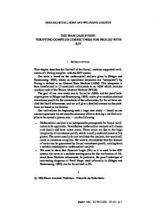
8.2 Inductive Reachability Judgment We want to annotate t with reachability information b, b′ : B such that whenever (L, V, {b} s) −→∗ (L′ , V ′ , {b′ } t) we have b → b′ . Reachability is a non-trival semantic property, hence undecidable. We define inductively the judgment reach in Figure 8. Reach considers the value of the condition expression e in the empty environment: JeK ∅. If JeK ∅ = ⊥, both cases are assumed to be reachable, which may overapproximate. Reach-Let propagates reachability information through let-bindings: If the let is reachable, then so is its successor. Reach-App ensures that whenever a function application is reachable, then the function is also reachable. Reach-Cond evaluates JeK∅, i.e. it evaluates the condition under the empty variable environment. If β(JeK∅) = false then reachability is not propagated into the consequence s1 . Propagation into the alternative s2 is treated similarily. Reach-Fun propagates reachability into t. The context Λ is extended with the reachability information of the function bodies f : b. The topmost premise ensures that the reachability information for all function bodies is sound.
8.3 Transformation and Correctness In Figure 10, we define a function uce that removes all code not marked reachable. If all functions from a mutually recursive function definition are removed, the funstatement is removed, too. Conditionals are removed if the value of the condition can be statically evaluated.
20
filterby : ∀XY, (X → B) → list X → list Y → list Y filterby p (x :: x′ ) (y :: y ′ ) = if px then y :: filterby p x′ y ′ else filterby p x′ y ′ filterby p _, _ = nil filter : ∀X, (X → B) → list X → list X filter p x = filterby p x x Figure 9: Definition of filter
uce : Ann Exp B → Exp uce (let x = η in s) = let x = η in (uce s) uce (if e then s1 else s2 ) = if JeK∅ = true then uce s1 else if JeK∅ = false then uce s2 else if e then (uce s1 ) else (uce s2 ) uce (f e) = f e uce e = e uce (fun F in t) = let F ′ = uceF F in if |F ′ | = 0 then uce t else fun F ′ in (uce t) uceF F = let K = filter (λ(x, {b} s). b) F in map (λ(x, s).(x, uce s)) K Figure 10: Definition of Unreachable Code Elimination
21
Definition 19 We define the proof relation Puce where A := B Param _ x x′ := x = x′ Arg a v v ′ := v = v ′ Idx a f f ′ := a = true ∧ f = f ′ Lemma 22 If dom Λ = dom F then F k Λ; Λ′ kPuce uceF F . Lemma 23 F = f x = {b} s → Param b F (uceF F ). Lemma 24 Suppose that it holds F ′ = uceF F and we have that (LF MV ; L, V, s) ∼r (LF ′ MV ′ ; L′ , V ′ , uce t) then (L, V, fun F in s) ∼r (L′ , V ′ , if |F ′ | = 0 then uce t else fun F ′ in uce t). Proof. If |F ′ | = 0, then F ′ = nil. After reducing only the left side one step via Sim-Expansion-Closed, the assumption solves the goal. Otherwise we reduce both sides one step (Lemma 2), and the assumption solves the goal. � Theorem 2 Let Λ ⊢ reach {true} s and L ∼r L′ :Puce Λ. Then: (L, V, s) ∼r (L′ , V, uce s). Proof. Induction on s and in each case inversion of reach. • The case for let follows from Sim-Let-Call and the inductive hypothesis. • The case for the conditional follows by Lemma 10 and the inductive hypotheses. • The application case follows from L ∼r L′ :Puce Λ with Lemma 17, after discharging premises: Note that Λf = true by inversion on reach, so Idx Λf f f holds by definition. Argument evaluation agrees, since parameters, and arguments and environments are identical. • The case for operation is trivial, since operation and environments are identical. • In the function definition case, let F ′ = uceF F . Lemma 24 lets us deal with both cases uniformly and requires (LF MV ; L, V, t) ∼r (LF ′ ME ; L′ , E, uce t) ′ ′ P < After applying the inductive hypothesis, we must show LF ME ; L ∼ r LF ME ; L : ′ Λ ; Λ. We apply Lemma 15 and discharge its premises by using Lemma 22 and Lemma 23. The remaining premise requires us to show from
LF ME ; L ∼r LF ′ ME ; L′ :P Λ′ ; Λ
(∗)
BdyP L,L′
that LF ME LF ′ ME (Λ′ ; Λ) ⊆ ∼r . Unfolding Bdy, we obtain Idx (Λ′ ; Λ) f f ′ and Ff = (x, s) and Ff′ ′ = (x′ , s′ ) and Arg Λ′f v v ′ . Unfolding those, we have to show (LF ME ; L, E[x 7→ v], s) ∼r (LF ′ ME ; L′ , E[x 7→ v], uce s) The inductive hypothesis solves the goal with (∗).
22
�
9 Dead Variable Elimination Dead variable elimination relies on a true liveness analysis. A variable is live if it is (potentially) used later on. A variable is true life, if it is used to compute a value that is live later on. True liveness requires a fixed-point computation, but is able to detect parameters of a function that do not contribute to the behavior of the function.
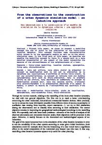
9.1 Inductive Liveness Judgement We specify sound true liveness information with the inductive judgment tlive in Figure 11. TLive-Op ensures that all variables that are live after the let (X ′ ) are also live before the let, except the variable defined. The free variables of e only need to be live if x is live after the let. TLive-Call is similar, but always requires the free variables of e to be live, as we can never remove calls (even if their result is unused). TLive-Exp requires the free variables of e to be live. TLive-Cond tests whether the condition is a constant expression by evaluating it in the empty environment. Only if this is unsuccessful, we require its free variables to be live. If β(JeK∅) 6= false, the consequence might be reachable. In this case the rule requires that all variables live in the consequence (X1 ) are live before the conditional (X1 ⊆ X), and that the judgment holds recursively. Otherwise, no requirements are imposed. TLive-App requires whenever a parameter xi is in the live set of the function body Xf , then the free variables of the corresponding argument expression ei are live at the application. TLive-Fun requires the liveness judgment to recursively hold for the continuation and the function bodies under extended contexts. The context ζ is extended with the parameters f : x of the newly defined functions, and the context Λ is extended with the liveness information f : Y for the function bodies. The rule requires all variables live after the function definition to be live before the function definition, and that all variables live in the function bodies (except parameters) are also live before the function definition.
9.2 Transformation and Correctness We realize dead variable elimination (DVE) with the recursive function dve defined in Figure 12. The recursive procedure descends through the program, removes unused let-bindings and filters parameter and argument lists according to liveness information. As in UCE, conditionals are removed if the condition can be statically evaluated. Definition 20 We define the proof relation Pdve where A := list V × set V Param (x, X) y y′ := x = y ∧ y ′ = filter (λx.x ∈ X) y Arg (x, X) v v ′ := v ′ = filterby (λ(x).x ∈ X) x v ∧ |x| = |v| Idx _ f f ′ := f = f ′
23
TLive-Op
X ′ \ {x} ⊆ X
TLive-Exp
x ∈ X ′ → fv(e) ⊆ X ζ | Λ ⊢ tlive {X ′ } s ζ | Λ ⊢ tlive {X} let x = e in {X ′ } s
fv(e) ⊆ X ζ | Λ ⊢ tlive {X} e
TLive-App
TLive-Call
X ′ \ {x} ⊆ X
|x| = |e| ′
fv(e) ⊆ X ζ | Λ ⊢ tlive {X } s ζ | Λ ⊢ tlive {X} let x = α e in {X ′ } s
∀i, xi ∈ Λf → fv(ei ) ⊆ X ζ | Λ ⊢ tlive {X} f e
TLive-Cond
JeK∅ = ⊥ → fv(e) ⊆ X β(JeK∅) 6= false → X1 ⊆ X ∧ ζ | Λ ⊢ tlive {X1 } s1 β(JeK∅) 6= true → X2 ⊆ X ∧ ζ | Λ ⊢ tlive {X2 } s2 ζ | Λ ⊢ tlive {X} if e then {X1 } s1 else {X2 } s2 TLive-Fun
f : x; ζ | f : Y ; Λ ⊢ tlive {X ′ } t ∀g, f : x; ζ | f : Y ; Λ ⊢ tlive {Yg } sg
X′ ⊆ X ∀g, Yg \ xg ⊆ X
ζ | Λ ⊢ tlive {X} fun f x = {Y } s in {X ′ } t Figure 11: Definition of the True Liveness Predicate ζ | Λ ⊢ tlive s. The context ζ : context (list V) contains parameters of functions, Λ : context (set V) contains the variables live in the function body, and s : Ann Exp (set V) is a program annotated with liveness information.
24
dve : list V → set V → Ann Exp (set V) → Exp dve ζ Λ (let x = e in {X} s) = let s′ = dve ζ Λ ({X} s) in if x ∈ X then let x = e in s′ else s′ dve ζ Λ (let x = α e in s) = let x = α e in (dve ζ Λ s) dve ζ Λ (if e then s1 else s2 ) = if JeK∅ = true then dve ζ Λ s1 else if JeK∅ = false then dve ζ Λ s2 else if e then (dve ζ Λ s1 ) else (dve ζ Λ s2 ) dve (ζ; f : x; ζ ′ ) (Λ; f : X; Λ′ ) ({_} f e) = f (filterby (λx.x ∈ X) x e) dve ζ Λ e = e dve ζ Λ (fun f x = {X} s in t) = let ∀i, Fi′ = (filter (λx.x ∈ Xi ) xi , dve (x; ζ) (X; Λ) si ) in fun F ′ in (dve (x, ζ) (X; Λ) t) Figure 12: Definition of Dead Variable Elimination
25
Lemma 25 If dom F = dom Λ = dom F ′ then we have F k Λ; Λ′ kPdve F ′ . Lemma 26 Let F = f x = {X} s and F ′ s.t. for all i, Fi′ = (filter (λx.x ∈ Xi ) xi , dve (x; ζ) (X; Λ) si ) and |F | = |F ′ |. Then Param (f : (x, X)) F F ′ . V =X V ′
We are now ready to show the correctness theorem. We write V =X V ′ agree on the values of the variables in the set X.
if V and V ′
< ′ Pdve Theorem 3 Let ζ | Λ ⊢ tlive {X} s and L ∼ zip ζ Λ and V =X V ′ . Then: r L :
′ ′ < (L, V, s) ∼ r (L , V , dve ζ Λ {X} s).
Proof. Induction on s and in each case inversion of tlive. • The case for let-call follows from Sim-Let-Call and the inductive hypothesis. • In the case for let op, we do a case analysis in x ∈ X. – If x ∈ X, the case follows from Sim-Let-Op with the fact that JeK V = JeK V ′ because V and V ′ agree on fv(e). – If x 6∈ X, case analysis on JeK V . ∗ If JeK V = ⊥, the left side is stuck (Sim-Error). ∗ If JeK V = v, we use Sim-Expansion-Closed to reduce the left side one step and are done by the inductive hypothesis with the observation that V [x 7→ v] still agrees with V ′ on the X because x 6∈ X. • The case for the conditional follows by Lemma 10 and the inductive hypotheses. • The case for application follows from L ∼r L′ :Pdve zip ζ Λ with Lemma 17, after discharging premises. The relation Idx (x, X) f f holds by definition. Argument evaluation agrees because Jfilterby (λx.x ∈ Xf ) x eK V ′ = filterby (λx.x ∈ Xf ) x (JeK V ) since we already know that JeK V 6= ⊥ and V and V ′ agree on the live variables. • The case for operation is trivial, since operation are identical and environments agree on the live variables. • In the function definition case, we have F ′ such that |F ′ | = |F | and for all i Fi′ = (filter (λx.x ∈ Xi ) xi , dve (x; ζ) (X; Λ) si ) We apply Lemma 16 and have to discharge premises. The second premise holds by assumption, the third is the inductive hypothesis. The first two requirements of the
26
first premise are Lemma 25 and Lemma 26. It remains to show from (∗)LF M; L ∼r LF ′ M; L′ :P (x, X; Λ) that ′ BdyP L,L′ F F ((x, X); Λ) ⊆ ∼r
After unfolding Bdy (Definition 13), we have the assumptions Idx (x, X) f f ′ and Ff = (x, s) and Ff′ ′ = (x′ , s′ ) and Arg (x, X) v v ′ . And after further unfolding we get x′ = filter (λx.x ∈ X) x and v ′ = filterby (λ(x).x ∈ X) x v. We have to show that (LF M; L, V [x 7→ v], s) ∼r (LF ′ M; L′ , V ′ [x′ 7→ v ′ ], dve (x; ζ) (X; Λ) s) Inductive hypothesis provides the latter. Its premises are discharged by (∗) and the observation that the updated environments still agree on the live variables. �
10 Coq Development The formal development accompanying this paper is part of a verified compiler LVC. LVC use the inductive method presented in this paper, and variations of it, for many correctness proofs. These include DVE, UCE, Copy Propagation, Sparse Conditional Constant Propagation, and some lowering passes. LVC also features an imperative variant of IL, which is called IL/I and serves as source language. The difference between IL and IL/I is that the latter uses imperative variables instead of lexically scoped binders. The first transformations in the pipeline of the LVC compiler are UCE and DVE on IL/I. The formal development hence also contains proofs of UCE and DVE for IL/I. The setup as described works for IL/I, too, and the proof structure remains the same. In the formal development we use De-Bruijn indices, not a named representation for function binders. This fact complicates UCE, as indices change whenever a function is removed. Fortunately, this does not causes problems with our inductive method. The part of the LVC development that pertains to this paper is available online: www.ps.uni-saarland.de/~sdschn/lvc-ind/ LVC has more than 36k LoC. The formalization of the inductive method (Section 6) takes ~400 LoC. The correctness theorems (Theorem 2, Theorem 3) are ~50 LoC each. Also counting lemmas, it takes ~300 LoC to show each of DVE and UCE correct.
11 Conclusion We described an inductive method for proofs of simulation-based program equivalence. In contrast to the standard approach, which indexes the (bi)simulation with a measure, our approach works without modifying the simulation. With out method, bisimilarity can be proven with the need for symmetrization.
27
After the method is setup, the overhead of the correctness proofs of transformations is low, and the proof becomes a straight-forward induction. The details of the proof are simple enough to be explained in full on paper. The method separates concerns: The correctness proofs follow the syntactic definition of the transformation, and a separate, general lemma proved by coinduction is used to deal with fixed-point computation in the language. This allows to focus on the actual verification problem inherent to the transformation instead of requirements induced by the proof method. We think inductive methods like ours are an essential tool for bisimulation-based compiler verification and useful in general. We applied the method to two optimizations, unreachable code elimination (UCE) and dead variable elimination (DVE). The optimizations are not straight-forward to verify because they remove instructions and change function signatures. The inductive method also improves modularity of the correctness argument: We argued certain removal steps in a separate lemma (e.g. Lemma 10). After using such a lemma in a plain coinductive proof (even when using Paco [3]), further justification would be required before the cohypothesis could be applied.
References [1]
Gilles Barthe, Delphine Demange, and David Pichardie. “A Formally Verified SSABased Middle-End - Static Single Assignment Meets CompCert”. In: ESOP. Vol. 7211. LNCS. Tallinn, Estonia, Mar. 24–Apr. 1, 2012.
[2]
Douglas J. Howe. “Proving Congruence of Bisimulation in Functional Programming Languages”. In: Inf. Comput. 124.2 (1996).
[3]
Chung-Kil Hur, Georg Neis, Derek Dreyer, and Viktor Vafeiadis. “The power of parameterization in coinductive proof”. In: POPL. Rome, Italy, Jan. 23–25, 2013.
[4]
Xavier Leroy. “A Formally Verified Compiler Back-end”. In: JAR 43.4 (2009).
[5]
Xavier Leroy. “Formal Verification of a Realistic Compiler”. In: CACM 52.7 (2009).
[6]
Robin Milner, Mads Tofte, and David Macqueen. The Definition of Standard ML. Cambridge, MA, USA: MIT Press, 1997.
[7]
Georg Neis et al. “Pilsner: a compositionally verified compiler for a higher-order imperative language”. In: ICFP. Vancouver, Canada, Sept. 1–3, 2015.
[8]
Scott Owens, Magnus O. Myreen, Ramana Kumar, and Yong Kiam Tan. “Functional Big-Step Semantics”. In: ESOP. Vol. 9632. LNCS. Eindhoven, The Netherlands, May 2– 8, 2016.
[9]
Sigurd Schneider. “Semantics of an Intermediate Language for Program Transformation”. Master’s Thesis. Saarland University, 2013. url: http://www.ps.uni-saarland.de/~sdschn/master.
[10]
Sigurd Schneider, Gert Smolka, and Sebastian Hack. “A Linear First-Order Functional Intermediate Language for Verified Compilers”. In: ITP. Vol. 9236. LNCS. Nanjing, China, Aug. 24–27, 2015.
[11]
Jaroslav Sevcík, Viktor Vafeiadis, Francesco Zappa Nardelli, Suresh Jagannathan, and Peter Sewell. “CompCertTSO: A Verified Compiler for Relaxed-Memory Concurrency”. In: J. ACM 60.3 (2013).
28
[12]
Jianzhou Zhao, Santosh Nagarakatte, Milo M. K. Martin, and Steve Zdancewic. “Formal Verification of SSA-based Optimizations for LLVM”. In: PLDI. Seattle, WA, USA, June 16–19, 2013.
29