Compiler optimization correctness by temporal logic ∗ David Lacey (
[email protected]) University of Warwick
Neil D. Jones (
[email protected]) University of Copenhagen
Eric Van Wyk (
[email protected]) University of Minnesota
Carl Christian Frederiksen (
[email protected]) University of Tokyo Abstract. Rewrite rules with side conditions can elegantly express many classical compiler optimizations for imperative programming languages. In this paper, programs are written in an intermediate language and transformation-enabling side conditions are specified in a temporal logic suitable for describing program data flow. The purpose of this paper is to show how such transformations may be proven correct. Our methodology is illustrated by three familiar optimizations: dead code elimination, constant folding, and code motion. A transformation is correct if whenever it can be applied to a program, the original and transformed programs are semantically equivalent, i.e., they compute the same input-output function. The proofs of semantic equivalence inductively show that a transformation-specific bisimulation relation holds between the original and transformed program computations.
1. Introduction This paper shows that temporal logic can be used to validate some classical compiler optimizations in a very strong sense. First, typical optimizing transformations are shown to be simply and elegantly expressible as conditional rewrite rules on imperative programs, where the conditions are formulae in a suitable temporal logic. In this paper the temporal logic is an extension of CTL with free variables. The first transformation example expresses dead code elimination, the second expresses constant folding and the third expresses loop invariant hoisting. The first involves computational futures, the second, computational pasts and the third, involves both the computational future and past. Second, the optimizing transformations are proven to be fully semantics-preserving: in each case, if π is a program and π 0 is the result ∗
This research was partially supported by the Danish Natural Science Research Council (PLT project), the EEC (Daedalus project) and Microsoft Research. c 2003 Kluwer Academic Publishers. Printed in the Netherlands. °
proving_final.tex; 3/11/2003; 21:26; p.1
of transforming it, an induction relation is established between the computations of π and π 0 . A consequence is that if π has a terminating computation with “final answer” v, then π 0 also has a terminating computation with the same final answer v; and vice versa. Compiler optimizing transformations: A great many program transformations are done by optimizing compilers; an exhaustive catalog may be found in (Muchnick, 1997). These have been a great success pragmatically, so it is important that there be no serious doubt of their correctness: that transformed programs are always semantically equivalent to those from which they were derived. Proof of transformation correctness must, by its very nature, be a semantics-based endeavor. 1.1. Semantics-based program manipulation Much has happened in this field since the path-breaking 1977 Cousot paper (Cousot et al., 1977) and 1980 conference (Jones (ed.), 1980). The field of “abstract interpretation” (Abramsky et al., 1987; Cousot et al., 1977; Cousot, 1981; Jones et al., 1994; Nielson, 1982; Nielson et al., 1999) arose as a mainly European, theory-based counterpart to the well-developed more pragmatic North American approach to program analysis (Aho et al., 1986; Hecht, 1977; Muchnick et al. (eds.), 1981). The goal of semantics-based program manipulation ((Jones, 1989) and the PEPM conference series) is to place program analysis and transformation on a solid foundation in the semantics of programming languages, making it possible to prove that analyses are sound and that transformations do not change program behaviors. This approach succeeded well in placing on solid semantic foundations some program analyses used by optimizing compilers, notable examples being sign analysis, constant propagation, and strictness analysis. An embarrassing fact must be admitted, though: Rather less success was achieved by the semantics-based approach toward the goal of validating correctness of program transformations, in particular, data-flow analysis-based optimizations as used in actual compilers. One root of this problem is that semantic frameworks such as denotational and operational semantics describe program execution in precise mathematical or operational terms; but representation of data dependencies along computational futures and pasts is rather awkward, even when continuation semantics is used. Worse, such dependency information lies at the heart of the most widely used compiler optimizing transformations. 2
1.2. Semantics-based transformation correctness
Transformation correctness is somewhat complex to establish, as it involves proving a soundness relation among three “actors”: the condition that enables applying the transformation and the semantics of the subject program both before and after transformation. Denotational and operational semantics (e.g., (Winskel, 1993)) typically present many example proofs of equivalences between program fragments. However most of these are small (excepting the monumental and indigestible (Milne et al., 1976)), and their purpose is mainly to illustrate proof methodology and subtle questions involving Scott domains or program contexts, rather than to support applications. A problem is that denotational and operational methods seem illsuited to validating transformations that involve a program’s computational future or computational past. Even more difficult are transformations that change a program’s statement ordering, notable examples being “code motion” and “strength reduction.” Few formal proofs have been made of correctness of such transformations. Two works relating the semantics-based approaches to transformation correctness: Nielson’s thesis (Nielson, 1981) has an unpublished chapter proving correctness of “constant folding” perhaps omitted from the journal paper (Nielson, 1982), because of the complexity of its development and proof. Havelund’s thesis (Havelund, 1984) carefully explores semantic aspects of transformations from a Pascal-like minilanguage into typical stack-based imperative intermediate code, but correctness proofs were out of its scope (and would have been impractically complex in a denotational framework, witness (Milne et al., 1976)). Cousot provides a general framework for designing program transformations whose analyses are abstract interpretations (Cousot et al., 2002), this framework is given at a higher level of generality than the proofs given in this paper, though in some ways the proofs could be seen as fitting into that framework. Some transformation correctness proofs have been made for functional languages, especially the sophisticated work by Wand and colleagues, for example (Steckler et al., 1997), using “logical relations.” These methods are mathematically rather more sophisticated than those of this paper, which seem more appropriate for traditional intermediate-code optimizations.
3
1.3. Model checking and program analysis This situation has improved with the advent of model checking approaches to program analysis (Cleaveland et al., 1997; Podelski et al., 2000; Schmidt, 1998; Schmidt et al., 1998; Steffen et al., 1995; Rus et al., 1998). Work by Steffen and Schmidt (Steffen, 1991; Steffen, 1993; Schmidt, 1998; Schmidt et al., 1998) showed that temporal logic is well-suited to describing data dependencies and other program properties exploited in classical compiler optimizations. In particular, work by Knoop, Steffen and R¨ uthing (Knoop et al., 1994) showed that new insights could be gained from using temporal logic, enabling new and stronger code motion algorithms, now part of several commercial compilers. More relevant to this paper: The code motion transformations could be proven correct. 1.4. Kleene algebra with tests Another approach to correctness of compiler optimizations is presented by Kozen and Patron (Kozen et al., 2000). Using an extension of Kleene algebra, Kleene algebra with tests (KAT), an extensive collection of instances of program transformations are proven correct, i.e., a concrete optimization is proven correct given a concrete source program and the transformed program. Programs are represented as algebraic terms in KAT and it is shown that the original and transformed program are equal under the algebraic laws of KAT. In many instances these terms are not ground, that is, they contain variables, and thus the reasoning could be applied to more general programs. One has to note that the paper sets out with a different perspective than ours on program transformation. It is geared towards establishing a framework where one can formally reason about program manipulations specified as KAT equalities that imply semantic equivalence. Unfortunately the results in the paper are not directly applicable to compilers since no automatic method is given for applying the optimizations described. In contrast, the present paper aims to formalize a framework for describing and formally proving classical compiler optimizations. We claim that these specifications (once proven correct) can be directly and automatically utilized in optimizing compilers. 1.5. Model checking and program transformation In this paper we give a formalism (essentially it is a subset of (Lacey et al., 2001)) for succinctly expressing program transformations, making 4
use of temporal logic; and use this formalism to prove the universal correctness (semantics preservation for all programs) of the three optimizing transformations: dead code elimination, constant folding and loop invariant hoisting. The thrust of the work is not just to prove these three transformations correct, though, but rather to establish a framework within which a wide spectrum of classical compiler optimizations can be validated. More instances of this paper’s approach may be found in the paper (Frederiksen, 2002), in the longer unpublished report (Frederiksen, 2001), and in the thesis (Lacey, 2003). The approach is similar to other approaches to specifying transformations and analyses together, for example in (Assmann, 1996; Whitfield et al., 1991; Whitfield et al., 1997). This paper shows how our method of specification is particularly useful when considering correctness. A recent development: Technical report (Lerner et al., 2002) was directly inspired by (Lacey et al., 2002). In essence it allows a small subset of our temporal program properties to be specified, but it has been more fully automated than this work, building on a platform described in (Lerner et al., 2002). One may regard their work as a “proof of concept and relevance” of our approach to compiler transformation correctness proofs. Many optimizing transformations can be elegantly expressed using rewrite rules of form: I =⇒ I 0 if φ, where I, I 0 are intermediate language instructions and φ is a property expressed in a temporal logic suitable for describing program data flow. Its reading (Lacey et al., 2001): If the current program π contains an instruction of the form I at some control point p, and if flow condition φ is satisfied at p, then replace I by I 0 creating the transformed program π 0 . The purpose of this paper is to show how such transformations may be proven correct. Correctness means that if a transformation changes any program π into a program π 0 , then the two programs are semantically equivalent, i.e., they compute the same input-output function. Section 4 shows how semantic equivalence can be established between π and π 0 .
2. Programs and their semantics In this section we provide fundamental definitions used in our representations of programs. In section 2.1 we introduce a simple imperative programming language that we use to demonstrate program transformations and their proofs of correctness. Section 2.2 defines the semantics of the language, including the notion of semantic equivalence which is key to defining the correctness of transformations. 5
0jj ¼
0: read x;
1j ?
1: five := 5;
2j ?
2: y := 0;
3j ?
3: c := five; 4: y := y + c * x; 5: x := x-1; 6: if x goto 4 else 7; 7: write y
4j ?
µ ? 5j ? 6j ?¼ 7jj
Figure 1. Example program and control flow graph.
2.1. A simple programming language Definition 1 A program π has the form: π
=
read x; I1 ; I2 ; ... Im−1 ; write y
where I1 , . . . , Im−1 are instructions. By convention every instruction has a unique label in Nodes π = {0, 1, 2, . . . , m}, with 0 labeling the initial read x and m labeling the final write y. Further, let instruction I0 be the initial read x, and instruction Im be the concluding write y. The read and write instructions must, and can only, appear respectively at the beginning and end of a program. The syntax of all other instructions in π is given by the following grammar: Inst
3
I
::=
Expr Op
3 3
E O
::= ::=
Var Label
3 3
X n, n0
::= ::=
skip | X := E | if X goto n else n0 X | O E...E various unspecified operators o, each with arity(o) ≥ 0 x | y | z | ... 1 | 2... | m
Program semantics is as expected and are formally defined below in Section 2.2. Figure 1 contains an example program. For readability it has explicit instruction labels, and operators are written in infix position. 6
In order to provide a simple framework for proving correctness this language has no exceptions or procedures. We expect the technique can be extended to include such features and maintain its fundamental nature, but this is future work. 2.2. Program semantics In this section we define the semantics of the simple programming language introduced in Definition 1. In Section 5 we use this semantics to show for a program π and its transformed version π 0 that their semantics are the same. That is, [[π]] = [[π 0 ]]. Definition 2 (Semantic framework) We assume the following have been fixed in advance, and apply to all programs: − A set Value of values (not specified here), containing a designated element true. − A fixed interpretation of every n-ary operator symbol o as a function [[o]]op : Value n → Value. Note that [[o]]op ∈ Value if n = 0. We assume that these functions are total. In Section 6.3 we discuss the issues raised by partial functions and exceptions, such as division by zero, and describe how our proof method is general enough to accommodate them. Definition 3 (Expression evaluation) A store is a function σ ∈ Store = Var * Value. Expression evaluation [[Expr ]]exp : Store → Value is defined by: [[X]]exp σ = σ(X) [[O E1 . . . En ]]exp σ = [[O]]op ([[E1 ]]exp σ, . . . , [[En ]]exp σ) Define σ\X to be the store function σ restricted to its original domain minus X. Further, σ[X 7→ v] is the same as σ except that it maps X to v ∈ Value. Definition 4 (Semantics) At any point in its computation, program π will be in a state of the form s = (p, σ) ∈ State π = N odesπ × Store. The initial state for input v ∈ Value is In(v) = (0, σ) where σ(x) = v and σ(Z) = true for all other variables appearing in program π. A final state is one that has the form (m, σ), where m is the label of the last instruction in π. The state transition relation → ⊆ State × State is defined by: 7
1. If Ip = skip or Ip = (read x) then (p, σ) → (p + 1, σ). 2. If Ip = (X := E) then (p, σ) → (p + 1, σ[X 7→ [[E]]exp σ]). 3. If Ip = (if X goto p0 else p00 ) and σ(X) = true then (p, σ) → (p0 , σ). 4. If Ip = (if X goto p0 else p00 ) and σ(X) 6= true then (p, σ) → (p00 , σ). Note that the read x has no effect on the store σ since the initial value v of x is set in the initial state. The operational semantics of a program is given the form of a transition system: the execution transition system Trun . Definition 5 A transition system is a pair T = (S, →), where S is a set and → ⊆ S × S. The elements of S are referred to as states or nodes. Definition 6 The execution transition system for program π and input v ∈ Value is by definition Trun (π, v) = (N odesπ × Store, →) where s1 → s2 is as in Definition 4. Definition 7 The semantic function [[π]] : Value * Value is the partial function defined by: [[π]](v) = σ(y) iff there exists a finite sequence from the initial state to a final state In(v) = s0 → s1 → . . . → st = (m, σ) In order to reason about the computational history of program executions we will also introduce the notion of computational prefix, and a corresponding transition system Tpfx (both defined in Section 4).
3. Analysis and transformation In section 3.1 we describe the control flow graph representation of programs that serves as the model over which the temporal logic formulae in the rewrite rules are checked. The temporal logic CTL with free variables is presented in section 3.2. The rewriting rules are defined in 8
section 3.3 and section 3.5 provides the specifications for the dead code elimination and constant folding transformations. 3.1. Modeling program control flow In order to reason about the program with a view to transform it, we look at the control flow graph of the program. This is type of transition system and it also an example of a model (as used in model checking). Models are transition systems where each state is labeled with certain information: Definition 8 A model (or Kripke structure (Kripke, 1963)) is a triple M = (S, →, L) (and a set of propositions P) where (S, →) is a transition system and labeling function L : S → 2P labels each state in S with a set of propositions in P. The control flow graph for program π is a system whose states are program points and whose transitions from one program point to another could occur consecutively in the execution. Definition 9 Tcf (π) = (Nodes π , →cf ) is the control flow graph for π, where the (total) relation →cf is defined by n1 →cf n2 if and only if (In1 ∨ (In1 ∨ (In1 ∨ (In1
∈ {X := E, skip, read x} ∧ n2 = n1 + 1) = if X goto n else n0 ∧ (n2 = n ∨ n2 = n0 ) ) = write y ∧ n2 = n1 ) = read x ∧ n2 = n1 )
Note that the self-loop transitions on the read and write nodes do not have corresponding transitions in the execution transition system Trun (π, v). They exist in Tcf (π) only to satisfy the totality requirement (in both arguments) of →cf imposed by CTL-FV, see Section 3.2 We will sometimes drop the cf subscript when it is clear that the control flow transition relation is being used. We set up a control flow model by labeling the states of the control flow graph (program points in this case) with propositions of interest. These will include the instruction at that program point plus information on which variables are defined or used at that point. Figure 2 shows the control flow model for the program in Figure 1 in which node 2, whose instruction y:=0 is labeled by the propositions node(2), stmt(y := 0), def (y), and conlit(0).
9
Nodes π = {0, 1, 2, 3, 4, 5, 6, 7} →cf = {0 →cf 0, 0 →cf 1, 1 → 2, 2 →cf 3, 3 →cf 4, 4 →cf 5, 5 →cf 6, 6 →cf 7, 6 →cf 4, 7 →cf 7} Lπ (0) Lπ (1) Lπ (2) Lπ (3) Lπ (4)
= = = = =
{node(0), stmt(read x), def (x)} ∪ trans 0 {node(1), stmt(five := 5), def (five), conlit(5)} ∪ trans 1 {node(2), stmt(y := 0), def (y), conlit(0)} ∪ trans 2 {node(3), stmt(c := five), def (c), use(five)} ∪ trans 3 {node(4), stmt(y := y + c ∗ x), def (y), use(y), use(c), use(x)} ∪ trans 4 Lπ (5) = {node(5), stmt(x := x − 1), def (x), use(x), conlit(1)} ∪ trans 5 Lπ (6) = {node(6), stmt(if x goto 4 else 7), use(x)} ∪ trans 6 Lπ (7) = {node(7), stmt(write y), use(y)} ∪ trans 7
Figure 2. Control flow model for the example program.
Definition 10 The control flow model for program π is defined as Mcf (π) = (Nodes π , →cf , Lπ ) where (Nodes π , →cf ) are as in Definition 9, and Lπ (n) is defined as follows for n ∈ Nodes π : Lπ (n)
where trans n
= ∪ ∪ ∪
{stmt(In ) {node(n)} {def (X) {use(X)
|
0 ≤ n ≤ m}
| |
∪ ∪
{use(Y) {conlit(O)
| |
In has form X:=E or read X} In form: Y:=E with X in E, or In = if X goto p else p0 } n = m and In = write Y} O is a constant in In , i.e., an operator with arity(O) = 0}
∪
trans n
=
{trans(E)
|
E is an expression in π and In is not of form: X:=E0 or read X with X in vars(E) }
The predicates stmt(I), def(X),use(X), conlit(O), trans(E) are the building blocks for the conditions that specify when optimizing transformations can be safely applied. These conditions are specified as CTL-FV 10
formulae. Note that trans(E) is the set of transparent expressions on a node: the expressions whose value is not changed by the node. 3.2. CTL with free variables
A path over → is an infinite sequence of nodes n0 → n1 → . . . such that ∀i ≥ 0 : ni → ni+1 . A backwards path is an path over the inverse of → (written as →◦ ) and is written as either n0 →◦ n1 →◦ . . . or n0 ← n1 ← . . .. The temporal logic CTL-FV used in specifying transformation conditions is in two respects a generalization of CTL (Clarke et al., 1986). First, as is common, the existential and universal temporal path quantifiers E and A are extended to also quantify over backwards paths in the ← − ← − obvious way. Our notation for this: E and A . We consider a branching notion of past which is infinite, as in P OT L (Pinter et al., 1984; Wolper, 1989) and not the finite branching past in CT Lbp (Kupferman et al., 1995). A branching past is more appropriate here than the linear past in P CT L∗ (Hafer et al., 1987) which can also be used to augment branching time logics with past time operators. Second, propositions are generalized to predicates over free variables. (A traditional atomic proposition is simply a predicate with no arguments.) For example, the formula stmt(x := e) where stmt is from the set P r of predicate names, has free variables x and e ranging over program variables and expressions, respectively. These free variables will henceforth be called CTL-variables to avoid confusion with variables or program points appearing in the program being transformed or analyzed. The effect of model checking will be to bind CTL-variables to program points or bits of program syntax, e.g., dead variables or available expressions. A CTL-FV formula is either a state formula φ or a path formula ψ, generated by the following grammar with non-terminals φ, ψ, terminals true, f alse, pr ∈ P r and free variables x1 , . . . , xn , start symbol φ and the productions: φ ::= true | false | pr(x1 , . . . , xn ) | φ ∧ φ | φ ∨ φ | ¬φ |
Eψ
ψ ::= X φ
| Aψ
← − | E ψ
| φU φ | φW φ 11
← − | A ψ
Operational interpretation: A model checker will not simply find which nodes in a model satisfy a (state) formula, but will instead find the instantiation substitutions that satisfy the formula. Mathematically, we model this by extending the satisfaction relation n |= φ to include a substitution θ binding its free variables. The extended satisfaction relation n |=θ φ is defined in Figure 3 and will hold for any θ such that n |= θ(φ). Here, θ(φ) is a standard CTL formula with no free variables and |= is as traditionally defined in (Clarke et al., 1986). Thus, the standard abbreviations from CTL, e.g. F φ ≡ true U φ, Gφ ≡ ¬F ¬φ and φ1 W φ2 ≡ (φ1 U φ2 ) ∨ Gφ1 , hold in CTL-FV as well. The job of the model checker is thus, given φ, to return the set of all n and θ such that n |=θ φ. For the example program in Figure 1 and formula def (x ) ∧ use(x), the model checker returns the following set of instantiation substitutions. (For brevity, CTL-variable n is bound to the program point in the substitutions.) {θ1 , θ2 } = {[n 7→ 4, x 7→ y], [n 7→ 5, x 7→ x]} Of particular interest when analyzing the control flow model is the universal weak until operator (A W ). Its use ensures that loops in the control flow model do not invalidate optimization opportunities where they can be safely applied, where as A U would. 3.3. Rewriting Definition 11 A rewrite rule has form: I =⇒ I 0 if φ, where I, I 0 are instructions built from program and CTL variables, and φ is a CTL-FV formula. By definition Rewrite(π, π 0 , n,I =⇒ I 0 if φ) is true if and only if for some substitution θ, the following holds: n |=θ stmt(I) ∧ φ π = read x; I1 ; ...In ;...Im−1 ; write y, where In = θ(I), and 0 0 π = read x; I1 ; ...θ(I ); ...Im−1 ; write y Sometimes we may want to alter the program at more than one point. In this case we specify several rewrites and side conditions at once. For example, to transform two nodes the form of the rewrite would be: n : I1 =⇒ I10 m : I2 =⇒ I20 if n |= φ1 m |= φ2 12
State Formulae: n |=θ n |=θ n |=θ n |=θ n |=θ n |=θ
true false pr(x1 , . . . , xn ) ¬φ φ1 ∧ φ 2 φ1 ∨ φ 2
n |=θ n |=θ n |=θ n |=θ
Eψ Aψ ← − E ψ ← − A ψ
iff iff iff iff
∃ ∀ ∃ ∀
path path path path
iff iff iff iff iff iff
true false pr(θx1 , . . . , θxn ) ∈ Lπ (n) not n |=θ φ n |=θ φ1 and n |=θ φ2 n |=θ φ1 or n |=θ φ2
(n = n0 → n1 → n2 . . .): (n = n0 → n1 → n2 . . .): (. . . n2 → n1 → n0 = n): (. . . n2 → n1 → n0 = n):
(ni )i≥0 (ni )i≥0 (ni )i≥0 (ni )i≥0
|=θ |=θ |=θ |=θ
ψ ψ ψ ψ
Path Formulae: (ni )i≥0 |=θ X φ iff n1 |=θ φ (ni )i≥0 |=θ φ1 U φ2 iff ∃k ≥ 0 : [nk |=θ φ2 ∧ ∀i : [0 ≤ i < k implies ni |=θ φ1 ]] (ni )i≥0 |=θ φ1 W φ2 iff (∃k ≥ 0 : [nk |=θ φ2 and ∀i : 0 ≤ i < k ⇒ ni |=θ φ1 ]) or (∀k ≥ 0 : [nk |=θ φ1 ]) Figure 3. CTL-FV satisfaction relation
The operational interpretation of this is that we find a substitution θ that satisfies both n |=θ stmt(I1 ) ∧ φ1 and m |=θ stmt(I2 ) ∧ φ2 and then use this substitution to alter the program at places n and m. 3.4. Computational aspects We discuss computational aspects only briefly; more can be found in (Lacey et al., 2001) and related papers. Model checking with respect to I =⇒ I 0 if φ yields a set of pairs {(p1 , θ1 ), . . . , (pk , θk )} satisfying φ. Consequence: {p1 , . . . , pk } is the set of all places where this rule can be applied. For instance, all immediately dead assignments can be found by a single model check. The time to model check n |= p for transition system T is a lowdegree polynomial, near linear for many transition systems, and |T |2 ·|φ| 13
in the worst case. Of course, in the case of model checking CTL-FV formulae times could be higher, since |T | depends on the size of labelling function L : Nodes π → 2AP as in Definition 10. For each node n, Lπ (n) can be found in time proportional at most to the size of the instruction In , with one exception: Propositions trans(E) can require time and space proportional to the size of π at each node n. For greater efficiency these can be treated specially, maintaining a single global data structure for the transparency relation. Experience from (Lacey et al., 2001) and related work indicates that their algorithm for model checking CTL-FV is not too expensive in practice, i.e., that the free variables do not impose an unreasonable time cost. 3.5. Sample transformations Following are versions of three classical optimizations (simplified in comparison to compiler practice, to make it easier to follow the techniques used in the proofs). We express code removal as replacement of an instruction by skip, and code motion as simultaneous replacement of an instruction I and skip by (respectively) skip and instruction I. This is convenient since it means the original and transformed programs have labels in a 1-1 correspondence. (We assume the compiler will remove useless occurrences of skip.) While most programmers do not write code that contains dead code or opportunities for constant folding, other transformations (especially automated ones) often enable these optimizations. Dead Code Elimination: Dead code elimination removes assignment statements that assign a value that is never used. In our model, the rewrite replaces the assignment with the skip instruction: x := e =⇒ skip The side condition on the rewrite must specify that the value assigned is never referenced again. This is exactly the kind of condition that temporal logic can specify. We can thus express dead code elimination as a rewrite rule with a side condition: x := e =⇒ skip if AX A( ¬use(x) W def (x) ∧ ¬use(x) ).
14
Since we do not care whether x is used at the current node, we skip past it with the AX operator. After this point we stipulate that x is never used again or not used until it is redefined (when def (x) holds). Constant Folding: A weak form of constant folding is a transformation to replace a variable reference with a constant value: x := y =⇒ x := c. One method of implementing constant folding for a variable Y is to check whether all possible assignments to Y assign it the same constant value. To check this condition we use the past temporal operators, specifying the complete transformation as follows1 : x := y =⇒ x := c if
← − A (¬def (y) ∧ ¬stmt(read x) W stmt(y := c) ∧ conlit(c)) The clause ¬stmt(read x) ensures that all paths from the entry read instruction to the instruction x := y contain an instruction x := c. Code motion/loop invariant hoisting: First, an example program, where the statement x:=a+b may be lifted from label 3 to label 1: 1: 2: 3: 4: 5: 6:
skip; if . . . then 3 else 6; x := a + b; y := y − 1; if y then 3 else 6; x := 0;
A restricted version of a “code motion” transformation (CM ) that covers the “loop invariant hoisting” transformation is defined as p q if p q
: skip =⇒ x :=e : x :=e =⇒ skip |= A(¬use(x) W node(q)) |= ¬use(x) ∧ ← − A ((¬def (x) ∨ node(q)) ∧ trans(e) ∧ ¬stmt(read x) W node(p))
This transformation involves two (different) statements in the subject program. The transformation moves an assignment at label q to label p provided that two conditions are met: 1
The conlit is introduced so that the model checker will not match c with a non-constant expression.
15
1. The assigned variable x is dead after p and remains so until q is reached. If this requirement holds, then introducing the assignment x:=e at label p will not change the semantics of the program. 2. The second requirement (in combination with the first rewrite rule) states that the expression e should be available at q after the transformation. This transformation could also be obtained by applying two transformations: One that inserts the statement x:=e provided that x is dead between p and q, followed by the elimination of available expressions transformation. With the two transformations one would need some mechanism of controlling where to insert which assignments. By formulating the transformation as a single transformation, the two labels p and q are explicitly linked. Since not all paths from p may eventually reach q, it is possible to move assignments to labels such that e is still available in q and x is dead in all paths not leading to q, which would still be a semantics preserving transformation. (In general the transformation by itself could slow down the computation, as is the case in our illustrating example, since there is no need to compute the expression if the expression is not needed; but this is not our point.) Note that we use the weak until (W ). This is so that the transformation is not disabled by cycles in the control flow graph that do not affect the correctness of the transformation.
4. A Method for Showing Semantic Equivalence Our method proves that the transformed program’s computations are bisimilar with those of the original. Definition 12 A bisimulation between transition systems T = (C, →) and T 0 = (C 0 , →0 ) is a relation R ⊆ C × C 0 such that if s ∈ C, s0 ∈ C 0 and sRs0 then 1. s → s1 implies s0 → s01 for some s01 with s1 Rs01 2. s0 → s01 implies s → s1 for some s1 with s1 Rs01 Transformation correctness: For each rewrite rule I =⇒ I 0 if φ we need to show that if Rewrite(π, π 0 , p,I =⇒ I 0 if φ), i.e., if π is transformed into π 0 then [[π]] = [[π 0 ]], meaning that for any input v, program π has a terminating computation In(v) →∗ (m, σ) if and only if program 16
π 0 has a terminating computation In(v) →∗ (m0 , σ 0 ) with σ(y) = σ 0 (y). The problem now is how to link the temporal property φ, which concerns “futures” and “pasts”, to the transformation I =⇒ I 0 . For this it is not sufficient to regard states one at a time, because the ← − operators A U and A U give access to information computed earlier or later. Our solution is to enrich the semantics and its transition system by considering computation prefixes of form: C = π, v ` s0 → . . . → st . Some informal remarks. Suppose we have model checked p |=θ φ on program π’s control flow graph. If φ contains only “past” operators, then the resulting substitutions also describe places in the computation prefix C where φ is true. Conclusion: The results of the model check contain information about the state sequence in C, thus relating past and present states. What about futures? Our choice is to define a prefix transition system Tpfx (π, v) so C → C1 ∈ Tpfx (π, v) if and only if C1 is identical to C, but with one additional state: C1 = π, v ` s0 → . . . → st → st+1 . Now reasoning that involves futures can be done by ordinary induction: assuming CRC 0 , show C → C1 implies C 0 → C10 for a C10 with C1 RC10 , and C 0 → C10 implies C → C1 for a C1 with C1 RC10 . Definition 13 For a program π and initial value v ∈ V alue, a computation prefix is a sequence (finite or infinite) π, v ` s0 → s1 → s2 → . . . such that s0 = In(v) and si → si+1 for i = 0, 1, 2, . . . A terminating computation prefix is one that reaches the read y instruction. Definition 14 The computation prefix transition system for program π and input v ∈ Value is by definition Tpfx (π, v) = (C, →) where C is the set of all finite computation prefixes, and C1 → C2 if and only if C1 = π, v ` s0 → s1 → . . . → st , C2 = π, v ` s0 → s1 → . . . → st → st+1 . 17
where st → st+1 is the state transition relation from Definition 4. Note that we use the same symbol, →, to represent both the transition relation for the execution transition system Trun and the computation prefix transition system Tpf x but that the relations can be distinguished by their context. Goal: Consider two programs, π and π 0 such that: π = read x; I1 ; I2 ; . . . Im−1 ; write y and
0 π 0 = read x; I10 ; I20 ; . . . Im 0 −1 ; write y.
The aim is to show that π and π 0 are semantically equivalent, [[π]] = [[π 0 ]]. That is, for any value v either both [[π]](v) and [[π 0 ]](v) are not defined or for any terminating computation prefix π, v ` In(v) → (p1 , σ1 ) → . . . → (m, σ) there exists a terminating computation prefix for the transformed program π 0 , v ` In(v) → (p01 , σ10 ) → . . . → (m0 , σ 0 ) such that σ(y) = σ 0 (y), and conversely. It is natural to try to prove this by induction on the length of computation prefixes. In practice the art is to find a relation R that holds between finite computation prefixes of the original program and those of the transformed program. R must be provable, and imply output equivalence for any program input v. More explicitly: If C, C 0 are computation prefixes of π, π 0 on the same input v, we show that si Rs0j for every corresponding pair of states in C, C 0 where R is a relation on states that expresses “correct simulation”. Remark: the transformations in this paper all satisfy m = m0 . Further, CRC 0 holds only if C, C 0 have the same length, and pi = p0i for any i. Thus CRC 0 implies that C → C1 for some C1 iff C 0 → C10 for some C10 . The following lemma details the work that needs to be done to show that semantic equivalence is preserved by any one step by the transition system. Lemma 1 (Program Equivalence/Induction) Programs π and π 0 are semantically equivalent, [[π]] = [[π 0 ]], if there exists a relation R, such that for all values v the following three conditions hold: 1. (Base Case) R holds between the initial computation prefixes i.e., [π, v ` In(v)] R [π 0 , v ` In(v)] 18
2. (Step Case) If C1 RC10 , C1 → C2 and C10 → C20 then C2 RC20 . 3. (Equivalence) If CRC 0 and C = π, v ` s0 → s1 . . . → (pt , σ) and C 0 = π 0 , v ` s00 → s01 . . . → (p0t0 , σ 0 ) then
(i) pt = m ⇐⇒ p0t0 = m and (ii) pt = p0t0 = m ⇒ σt (y) = σt0 0 (y)
Proof. Straightforward by two inductions. Proofs of equivalence are split into these three steps. This schema of proof provides a “top-level” approach to proving the correctness of optimizations. The questions still remain however of how to determine the relation R and how to prove the conditions of Lemma 1. In particular, it is the “step case” that is hardest to prove. The relation R will clearly be derived from the CTL-FV side conditions of the transformations. Imagine we are defining R as a relation that holds between two computation prefixes C and C 0 where: C = π, v ` s0 → s1 → . . . → st , C 0 = π 0 , v ` s00 → s01 → . . . → s0r for some programs π,π 0 and initial value v. Let si = (pi , σi ) and s0i = (p0i , σi0 ) for all i ≥ 0. Consider the case where we have a side condition p |= A(φ1 U φ2 ) or p |= A(φ1 W φ2 ). A complete (terminating) trace that contains p = pi will have the following form: φ2 holds ↓
prior to until z
}|
{
after until z
}|
{
s0 → . . . → si−1 → si → . . . → st−1 → st → st+1 → . . . → sw |
{z
}
until section: φ1 holds
The computation is split into an “until section” and sections that are outside the until. For non-terminating computational prefixes, the last state of the prefix may also be in the until section. In the case of p |= A(φ1 W φ2 ), the until section may continue to the end of a terminating computation prefix with φ2 never holding. The relation R will depend on this; either the last state of a computation prefix is within an until section and one condition, say A, holds or it is outside this section and 19
a different condition, say B, holds. The relation R for transformations with A U or A W side conditions will naturally have the form where one of the following two cases hold: − A − ∃i : i < t ∧ pi = p ∧ (∀j : i ≤ j < t ⇒ pj |= ¬φ2 ) and B Here A and B are conditions chosen depending on the transformation and the formulae φ1 and φ2 in the temporal side condition (see the examples in the next section). What about backwards until and waits-for formulae? In this case, ← − ← − where p |= A (φ1 U φ2 ) or p |= A (φ1 W φ2 ) is a side condition, we need to show as part of the relation R that being inside an until section preserves some property that can be used when leaving this section. So (in addition to some other conditions) the following will hold: − (∃i : i < t ∧ pi |= φ2 ∧ (∀j : i < j ≤ t ⇒ pj |= φ1 )) ⇒ A A complete trace that contains p = pt will have the following form: φ2 holds ↓
prior to until z
}|
{
after until z
}|
{
s0 → . . . → si−1 → si →. . . → st−1 → st → st+1 → . . . → sw |
{z
}
until section: φ1 holds
Here A will again depend on the transformation and the formula φ1 and φ2 . As before, in the case of the waits-for side condition, φ1 may hold all the way to the beginning of the computation prefix with φ2 never holding. If the relation R follows these schemata then in conjunction with the side conditions of the transformation it will provide information about the last state of the computation prefix during the step case of the proof. This information will allow us to prove that the relation holds of the prefixes extended by one state. The following two lemmas show how until formulae together with other conditions on a computation will indicate that a particular condition holds of the current state in a computation. The first says that p |= A(φ1 W φ2 ) implies that if φ2 has never been true since p, then φ1 has always been true since p. The second is its reverse-time analog of this result. Lemma 2 Suppose π, v ` (p0 , σ0 ) → . . . → (pt , σt ) is a computation prefix and we know that 20
p |= A(φ1 W φ2 ) and ∃i : i < t ∧ pi = p ∧ (∀j : i ≤ j < t ⇒ pj |= ¬φ2 ) and pt |= ¬φ2 . Then pt |= φ1 . Proof. Straightforward from the definition of CTL-FV. Lemma 3 Suppose π, v ` (p0 , σ0 ) → . . . → (pt , σt ) is a computation prefix and we know that ← − p |= A (φ1 W φ2 ) and (∃i : i < t ∧ pi |= φ2 ∧ (∀j : i ≤ j < t ⇒ pj |= φ1 )) ⇒ A and ∃i < t : pi |= ¬φ1 and pt = p . Then A will hold. Proof. Straightforward from the definition of CTL-FV. These two lemmas along with the side conditions of the transformation and the relation R will provide information about the current state of the computation. Given this information the table in Figure 4 shows how this will affect the next state of the computation. This will enable us to complete the step case of the proof. The following lemma shows how Figure 4 can be used. Lemma 4 Suppose (σt , pt ) is a state of π, (σt0 , p0t ) is a state of π 0 and 0 , p0 Ipt = Ip0 0 . If (σt , pt ) → (σt+1 , pt+1 ) and (σt0 , p0t ) → (σt+1 t+1 ) then t the contents of a table entry in Figure 4 will be true if pt satisfies the condition in the row header of the table and the states satisfy the condition in the column header (note that a “ ?” signifies that nothing significant holds of the next states). Proof. Tedious but straightforward from CTL-FV and Definition 4. Now we have a uniform method for proving that a transformation is correct. The following seven steps are to be followed: 21
¬def (x)
trans(e)
def (x)∧ ¬use(x) ¬use(x) T rue
σt = σt0 0 σt+1 = σt+1 pt+1 = p0t+1 σt+1 (x) = σt (x) 0 (x) = σ 0 (x) σt+1 t 0 (x) σt+1 (x) = σt+1 0 σt+1 = σt+1 0 pt+1 = pt+1 [[e]]exp σt = [[e]]exp σt+1 = 0 [[e]]exp σt+1 = [[e]]exp σt0 0 σt+1 = σt+1 0 pt+1 = pt+1 0 σt+1 = σt+1 0 pt+1 = pt+1 0 σt+1 = σt+1 0 pt+1 = pt+1
σt \ x = σt0 \ x
σt (x) = σt0 (x)
σt+1 (x) = σt (x) 0 (x) = σ 0 (x) σt+1 t
σt (x) = σt+1 (x) = 0 (x) = σt+1 σt0 (x)
[[e]]exp σt+1 = [[e]]exp σt 0 [[e]]exp σt+1 = [[e]]exp σt0
?
0 σt+1 = σt+1 0 pt+1 = pt+1 0 σt+1 \ x = σt+1 \x 0 pt+1 = pt+1
?
? ? ?
Figure 4. Local pre/post conditions
1. Choose a relation R based on the side conditions of the transformation. 2. Use Lemma 1 to reduce the proof into 3 steps: the base case, the step case and the final equivalence step. 3. The base case is usually trivial. 4. For the step case: split into different cases depending on whether we are at the point of transformation and whether we are entering or leaving an until section. 5. If appropriate use Lemmas 2 and 3 to determine the conditions true in the current state. 6. Use the pattern of the rewrite or Lemma 4 to complete the step case of induction. 7. Finish by proving the third part of Lemma 1. The next section provides three example proofs using this method. 22
5. The Three Examples 5.1. Dead Code Elimination The dead code elimination rewrite rule described earlier was: x := e =⇒ skip if AX A( ¬use(x) W (def (x) ∧ ¬use(x) ). Following Definition 11 of rewriting, for this rewrite to apply the model checker must find a particular program point p and a substitution that maps x to a particular program variable X and e to a particular expression E. In this case we need to prove that an original program π and transformed program π 0 are equivalent. Below, we assume that Rewrite(π, π 0 , p, x:=e =⇒ skip if AX A(¬use(x) W def (x)∧¬use(x) )) To prove that these two programs are equivalent we will use the method described in Lemma 1. However, to do this we need to come up with a relation R which holds between the two programs and ensures that the return value of the programs will be the same. To arrive at this relation we can examine the side condition of the transformation2 : AX A( ¬use(X) W def (X) ∧ ¬use(X) ) A key sub-formula in this condition is def (X) ∧ ¬use(X) which, for brevity, shall be abbreviated in this proof to φ2 (following the schema in the previous section). We can see from this condition that any label immediately following p will satisfy the formula A(¬use(x) W φ2 ) and this gives us a schema for the relation R (as described in the previous section) where one of the following two conditions holds: − A − ∃i : i < t ∧ pi = p ∧ (∀j : i ≤ j < t ⇒ pj |= ¬φ2 ) and B The question remains of what the conditions A and B should be. Outside of the until section we will know nothing about the program, so to ensure the return values are the same we need to stipulate that the store of the original program and its transformed version are the same i.e A ≡ σt = σt0 . Within the until section we can see that ¬use(X) will hold, this suggests (see Figure 4) that B ≡ σt \ X = σt0 \ X. 2
Note here that we have “substituted in” the values of the meta-variables in the formula.
23
Definition 15 Consider C ∈ Tpfx (π, v) and C 0 ∈ Tpfx (π 0 , v) such that: C = π, v ` s0 → s1 → . . . → st , C 0 = π 0 , v ` s00 → s01 → . . . → s0r in which ∀i : [0 ≤ i ≤ t ⇒ si = (pi , σi )] and ∀i : [0 ≤ i ≤ r ⇒ s0i = (pi , σi0 )]. Then CRC 0 if and only if t = r, pt = p0t and one of the following two cases holds: 1. σt = σt0 . 2. ∃j : j < t ∧ p = pj ∧ ∀k : j < k < t ⇒ pk |= ¬φ2 and σt \ X = σt0 \ X. 3 Having defined a suitable R we can then proceed to prove the correctness of dead code elimination using the method laid out in the previous section. Proof (Dead code elimination satisfies the conditions of Lemma 1). Base Case: For any initial prefixes: σt = σt0 , so CRC. Step Case: Suppose C1 RC10 and neither is terminated. The language is deterministic so C1 → C2 and C10 → C20 for exactly one C2 and C20 . We need to show that C2 RC20 . By Definition 15: C1 = π, v ` (p0 , σ0 ) → . . . → (pt , σt ) C10 = π 0 , v ` (p0 , σ00 ) → . . . → (pt , σt0 ) Let Ip be the instruction in program π at p and Ip0 be the instruction in program π 0 at p. To prove that C2 RC20 we need to split the situation into several different cases based on whether we are at the point of transformation (pt = p) or if we are potentially leaving the until section of the computation (pt |= φ2 ). There follows the proofs for every part of the case split: − Case 1: pt = p
⇒
C1 RC10 ∧ pt = p { Definition of R } σt \ X = σt0 \ X ∧ pt = p
3
Note that this is stronger than the condition in the schema presented earlier in that we’ve replaced the first ≤ in the ∀ with a