An Intelligent Flow Measurement Technique using Ultrasonic Flow ...

International Journal of Control and Automation Vol. 5, No. 4, December, 2012

An Intelligent Flow Measurement Technique using Ultrasonic Flow Meter with Optimized Neural Network Santhosh KV and BK Roy Department of Electrical Engineering, NIT, Silchar, India [email protected], [email protected] Abstract Design of an intelligent flow measurement technique using ultrasonic flow meter is reported in this paper. The objective of the work are; (i) to extend the linearity range of measurement to 100% of the input range, (ii) to make the measurement system adaptive to variations in pipe diameter, liquid density, and liquid temperature, and (iii) to achieve the objectives (i) and (ii) by an optimal Artificial Neural Network ((ANN). An optimal ANN is considered by comparing various schemes and algorithms based on minimization of Mean Square Error (MSE) and Regression close to one. The output of ultrasonic flow meter is frequency. It is converted to voltage by using a frequency to voltage converter. An optimal ANN block is added in cascade to frequency to voltage converter. This arrangement helps to linearise the overall system for 100% of full scale and makes it adaptive to variations in pipe diameter, liquid density, and liquid temperature. Since the proposed intelligent flow measurement technique produces output which is adaptive to variations in pipe diameter, liquid density, and liquid temperature, the present technique avoids the requirement of repeated calibration every time there is change in liquid, and/or pipe diameter, and/or liquid temperature. Simulation results show that proposed measurement technique achieves the objectives quite satisfactorily. Keywords: Artificial Neural Network, Optimization, Sensor modeling, Temperature compensation, Ultrasonic flow meter

1. Introduction Flow measurement has evolved over the years in response to measure new products, measure old products with new condition of flow, and for tightened accuracy requirement as the value of the fluid is gone up. Flow measurement is the quantification of bulk fluid movement. Flow can be measured in a variety of ways, may be by contact type or non-contact type of sensor. Positive-displacement flow meters accumulate a fixed volume of fluid and then count the number of times the volume is filled to measure flow. Other indirect flow measurement methods rely on forces produced by the flowing stream as it overcomes a known constriction. Flow may be measured by measuring the velocity of fluid over a known area. Accurate flow measurement is an essential requirement both from qualitative and economic points of view. Among the non contact type of flow measurement, ultrasonic flow measurement is widely used to measure flow, because of its advantage like high resolution and less interference of noise on output. However, non linear characteristics of Ultrasonic flow meters (UFM) have restricted its use. To overcome the restriction faced due to nonlinear response characteristics of the ultrasonic flow meter, several techniques have been suggested. But some of these are tedious and time consuming. Further, the process of calibration needs to be repeated or calibration circuit needs to be replaced/ tuned every time there is a change in pipe diameter or liquid

185

International Journal of Control and Automation Vol. 5, No. 4, December, 2012

density. The problem of nonlinear response characteristics of an UFM further aggravates when there is a change in liquid temperature, since the output of an UFM is dependent on temperature also. To overcome the above difficulties, an intelligent flow measurement technique is proposed in this paper. The optimal ANN is achieved considering different algorithms and schemes and comparing their least MSE and Regression close to one. This optimized ANN is used to train the system to obtain linearity and makes the output adaptive to variations in pipe diameter, liquid density, and liquid temperature, all within a range. Literature review suggests that several techniques are adopted to calibrate the UFM. In [1], linearization of UFM with the help of neural network algorithm is done. In [2], [4-7] calibration of flow meter using several hardware circuits is discussed. In [3] design of UFM is discussed in order to achieve maximum accuracy and implementation of microcontroller to linearise the output. In [8] linearization of UFM and making its output independent of physical parameters using ANN is discussed. The paper is organised as follows: Introduction in Section 1, is followed by a brief description on ultrasonic flow meter in Section 2. A brief discussion on data conversion i.e. a Frequency to voltage converter is discussed in Section 3. Section 4 deals with the problem statement which is followed by proposed solution in Section 5. Finally, results and conclusion are included in Section 6.

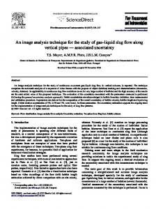
2. Ultrasonic Flow Meter Ultrasonic flow meters have gained a lot of attention over the past years, primarily because of their ability for measuring custody transfer of natural gas. They are replacing differential pressure and turbine flow meters in many natural gas applications. UFMs are also widely used to measure liquid flow. This is not limited to clean liquids either. A special type of UFM can accurately measure the flow of slurries and liquids with many impurities Ultrasonic flow meters are one of the most interesting types of meters used to measure flow in pipes. The most common variety, transit time, has both a sending and a receiving transducer. Figure 1 shows the arrangement of one such UFM. Both sending and receiving transducers are mounted on either side of the flow meter, or the pipe wall. The sending transducer sends an ultrasonic signal at an angle from one side of the pipe which is received by the receiving transducer. The flow meter measures the time that the ultrasonic signal takes to travel across the pipe in forward and reverse direction. When the signal travels along the direction of the flow, it travels more quickly compared to the condition of no flow. On the other hand, when the signal travels against the direction of flow, it slows down. The difference between the “transit times” of the two signals is proportional to flow rate [5, 1013].

Figure 1. Ultrasonic Flow Meter

186

International Journal of Control and Automation Vol. 5, No. 4, December, 2012

From Figure 1, we have

(1)

(2) ΔT = Tup - Tdown

(3)

Frequency, fIN = 1/ΔT where: M – No of times ultrasonic signal travels in forward/ backward direction Co – Velocity of ultrasonic signal in static fluid D – pipe diameter V – Velocity of fluid The velocity of ultrasonic signal depends on [13] density of liquid as,

(4) with

k – bulk modulus and ρ – Density of liquid

Effect of temperature on density [14-15] can be given by (5) where: ρ1 – specific density of liquid at temperature t1 ρ0 - specific density of liquid at temperature t0 Pt1 – pressure at temperature t1 Pt0 – pressure at temperature t0 E– Modulus of elasticity of the liquid α – temperature coefficient of liquid

3. Data Conversion Unit The block diagram representation of the proposed technique is given in Figure 2.

187

International Journal of Control and Automation Vol. 5, No. 4, December, 2012

Figure 2. Block Diagram of the Proposed Measuring Technique The LM2917 series is a monolithic frequency to voltage converters with high gain op amp/comparator designed to operate a relay, lamp, or other load when the input frequency reaches or exceeds a selected rate [16]. The op amp/comparator is fully compatible with the sensors and has a floating transistor as its output. The collector may be taken above VCC up to a maximum VCE of 28V. VOUT = fIN *R*C*VCC

(6)

Figure 3. Frequency to Voltage Converter Circuit using LM 2917

4. Problem Statement In this section, characteristic of ultrasonic flow meter is simulated to understand the difficulties associated with the available measurement technique. For this purpose, simulation is carried out with three different pipe diameters. These are D = 0.1 m, 0.2 m, and 0.3 m. Three different liquid densities are considered. These are ρ = 500 Kg/m3, 1000 Kg/m3, and 1500 Kg/m3. Three different liquid temperatures are considered. These are t = 25 oC, 50 oC, and 75 oC. The output frequency of UFM is calculated using Eq. 3, 4, and 5, with respect to various values of input flow considering a particular pipe diameter, liquid density, and temperature. These output frequencies are used as input of frequency to voltage converter circuit and by using Eq. 6, the output voltages are generated. The MATLAB environment is used of and the following characteristics are found.

188

International Journal of Control and Automation Vol. 5, No. 4, December, 2012

Figure 4. Output of Data Conversion Unit for Various Flow Rates and Temperatures at Liquid Density is 500 Kg/m3 and Pipe Diameter is 0.1 m

Figure 5. Output of Data Conversion Unit for Various Flow Rates and Liquid Densities at Temperature is 50 0C and Pipe Diameter is 0.3 m

Figure 6. Output of Data Conversion Unit for Various Flow Rates and Pipe Diameters at Liquid Density is 1500 Kg/m3 and Temperature is 75 0C Figure 4, Figure 5, and Figure 6 show the variation of voltages with the change in flow rate considering different values of pipe diameter, liquid density, and liquid temperature. It has been observed from the above graphs that the output from the frequency to voltage converter circuit has non linear relation. Datasheet of ultrasonic suggests that 10% to 50% of full scale input range is used in practice. The output voltage varies with the changes in pipe diameter,

189

International Journal of Control and Automation Vol. 5, No. 4, December, 2012

liquid density, and liquid temperature. These are the reasons which have made the user to go for repeated calibration techniques using some circuits. But, these conventional techniques have drawbacks that these are time consuming and need to be calibrated every time whenever pipe diameter, and/or liquid density, and/or liquid temperature are changed in the system. Further, the use is restricted only to a portion of full scale input range. To overcome these drawbacks, this paper makes an attempt to design a flow measurement technique using UFM incorporating intelligence to produce linear output and to make the system adaptive to variations in pipe diameter, liquid density, and liquid temperature using the concept of a neural network by taking an optimized ANN model. Problem statement: given an arrangement for measurement of flow consisting of UFM in cascade with frequency to voltage converter circuit, design an intelligent non contact flow measurement technique using optimized neural network model and having the following properties: i.

Adaptive to variation in diameter of the pipe.

ii.

Adaptive to variation in liquid density.

iii.

Adaptive to variation in liquid temperature.

iv.

Output bears a linear relation with the input flow rate.

v.

Full scale input range can be measured.

5. Problem Solution The drawbacks discussed in the earlier section are overcomed by adding an optimal ANN model in cascade with data converter unit. This model is designed using the neural network toolbox of MATLAB. The first step in developing a neural network is to create a database for its training, testing and validation. The output voltage of data conversion unit for a particular flow, pipe diameter, liquid density, and liquid temperature is stored as a row of input data matrix. Various such combinations of input flow, pipe diameter, liquid density, liquid temperature, and their corresponding voltages at the output of data conversion unit are used to form the other rows of input data matrix. The output matrix is the target matrix consisting of data having a linear relation with the flow and adaptive to variations in pipe diameter, liquid density, and liquid temperature, as shown in Figure 7.

Figure 7. Target Graph The process of finding the weights to achieve the desired output is called training. The optimized ANN is found by considering different algorithms with variation in the number of

190

International Journal of Control and Automation Vol. 5, No. 4, December, 2012

hidden layer. Mean Squared Error (MSE) is the average squared difference between outputs and targets. Lower value of MSE is better. Zero means no error. Regression (R) measures the correlation between output and target. Regression equal to 1 means a close relationship and 0 means a random relationship. Four different schemes and algorithms are used to find the optimized ANN. These are Levenberg-marquardt algorithm (LMA) [17, 18], Artificial Bee Colony (ABC) [19, 20], Ant colony optimization (ACO) [21, 22], Back Propagation neural network (BP) trained by Ant Colony Optimization (ACO) [21, 23]. Training of ANN is first done assuming only one hidden layer. MSE and R values are noted. Hidden layer is increased to 2 and training is repeated. This process is continued up to 4 hidden layers. In all cases, MSE and R are noted and are shown in Table 1. Mesh of MSE’s and R’s corresponding to different algorithms and hidden layers are shown in Figure 8 and Figure 9. From Table 1, Figure 8, and Figure 9, it is very clear that BP trained by ACO yields most optimized network assuming desired MSE as threshold. BP trained by ACO with 2 hidden layers is considered as the most optimized ANN for desired accuracy of result, as shown in Figure 10. Table 1. Comparison of Number of Hidden Layer with R and MSE

Figure 8. Mesh Showing the MSE Corresponding to Different ANN Models

191

International Journal of Control and Automation Vol. 5, No. 4, December, 2012

Figure 9. Mesh Showing the R Corresponding to Different ANN Models

Figure 10. Structure of Neural Network Model The network is trained, validated and tested with the details mentioned above. Table 2 summarizes the various parameters of the optimized neural network model. Table 2. Summary of the Network Model

Input

OPTIMIZED PARAMETERS OF THE NEURAL NETWORK MODEL Training base 120 Validation base 40 Database Test base 40 1st layer 8 No of neurons in 2nd layer 8 1st layer tansig Transfer 2nd layer tansig function of Output layer linear

192

Flow rate

D

ρ

Temp

min

0 m /s

0.1 m

500 Kg/m

25 oC

max

0.0025 m3/s

0.3 m

1500 Kg/m3

75 oC

3

3

International Journal of Control and Automation Vol. 5, No. 4, December, 2012

6. Results and Conclusion The optimized ANN is trained, validated and tested with the simulated data. It is subjected to various test inputs corresponding to different pipe diameters, liquid densities, and temperatures of liquid, all within the respective specified ranges. For testing purposes, the range of flow is considered from 0.0 to 0.0025m3/s, range of pipe diameter is 0.1 to 0.3 m, range of liquid density is 500 to 1500 Kg/m3, and liquid temperature is 25 to 75 oC. The flow measured by the proposed technique corresponding to sample test inputs are tabulated in Table 3. It shows that the actual flow rates and the measured flow rates by the proposed technique are same. The input-output result is plotted and is shown in Figure 11. The output graph is matching the target graph which is shown in Figure 8. Table 3. Result of Measuring System using Optimal ANN Actual flow in m3/s 0.0005 0.0005 0.0005 0.0010 0.0010 0.0010 0.0015 0.0015 0.0015 0.0020 0.0020 0.0020 0.0025 0.0025 0.0025

D in m 0.1 0.2 0.3 0.25 0.15 0.1 0.2 0.15 0.3 0.3 0.25 0.15 0.13 0.22 0.3

ρ in Kg/m3 500 1000 1500 1200 1100 900 800 700 600 500 750 1450 1300 1200 1150

t in o C 25 36 72 56 38 42 50 62 75 29 36 54 38 71 50

Data conversion o/p in V 2.5133 3.0953 4.0326 1.8525 0.0277 1.7406 1.3240 1.0450 3.3954 2.1703 1.2186 0.0514 0.4743 0.5734 0.8463

ANN o/p in V 1.0 1.0 1.0 2.0 2.0 2.0 3.0 3.0 3.0 4.0 4.0 4.0 5.0 5.0 5.0

Measured flow in m3/s 0.0005 0.0005 0.0005 0.0010 0.0010 0.0010 0.0015 0.0015 0.0015 0.0020 0.0020 0.0020 0.0025 0.0025 0.0025

Figure 11. Response of Proposed Measuring Technique It is evident from Figure 11 and Table 3 that the proposed measurement technique has gained intelligence in addition to increase in the linearity range. The output is made adaptive to variations in pipe diameter, liquid density, and liquid temperatures. Thus, if the liquid is changed by another liquid of different density, and/or the pipe is replaced by another pipe of

193

International Journal of Control and Automation Vol. 5, No. 4, December, 2012

different diameter, and/or liquid temperature is changed then the calibration process need not be repeated. Available reported works have discussed different techniques for calibration of flow measurement, but these are not adaptive to variations in pipe diameter, liquid density, and liquid temperature. Hence, repeated calibration is required for any change in pipe, or liquid, or liquid temperature. Sometime, the calibration circuit may itself be replaced which is a time consuming and tedious procedure. Further, some reported works have not utilized the full scale of measurement. In comparison to these, the proposed measurement technique achieves linear input-output characteristic for full scale input range and makes the output adaptive to variations in pipe diameter, liquid density, and liquid temperature. All these have been achieved by using an optimal ANN. Four different schemes and algorithm are used for training, validation and testing. BP using ACO is found to have achieved the desired MSE and Regression close to one with only two hidden layers. This is in contrast to an arbitrary ANN in most of the earlier reported works.

References [1] T. T. Yeh, P. I. Espina and S. A. Osella, “An Intelligent Ultrasonic Flow Meter for Improved Flow Measurement and Flow Calibration Facility”, Proc. IEEE Conf. On Instrument and Measurement Technology, Budapest, Hungary, (2001), pp. 1741-1746. [2] E. Aziz, Z. Kanev, M. Barboucha, R. Maimouni and M. Staroswiecki, “An ultrasonic flowmeter designed according to smart sensors concept”, Proc. IEEE 8th Mediterranean Electro technical conference, France, (1996), pp. 1371-1374. [3] J. Yang and H. Jiao, “Design of Multi-channel Ultrasonic Flowmeter based on ARM”, Proc. IEEE Conf. on Electrical and Control Engineering, Yichang, China, (2010), pp. 758-761. [4] L. Z. Yang, Z. Zhang and Dongsheng, “The Experiment Study of Ultrasonic Flowmeter Precision”, Journal of Xi’an University of Technology, vol. 22, no. 1, (2006), pp. 70-72 . [5] L. Guowei and C. Wuchang, “The Measurement Technology of Flow Rate and Instrument”, China Machine Press, (2002) June. [6] O. Keitmann-Curdes and B. Funck, “A new calibration method for ultrasonic clamp-on transducers”, IEEE Symposium on Ultrasonic’s, Berlin, (2008), pp. 517-520. [7] P. I. Espina, P. I. Rothfleisch, T. T. Yeh and S. A. Osella, “Telemetrology and advanced ultrasonic flow metering”, Proc. of the 4th International Symposium on Fluid Flow Measurement, Denver, USA, (1999). [8] Santhosh KV and BK Roy, “An Intelligent Flow Measuring Scheme Using Ultrasonic Flowmeter”, 31st International Conference on Modelling, Identification and Control (2012) April, Thailand. [9] L. C. Lynnworth, “Ultrasonic measurements for process control”, Academic Press, San Diego, CA, (1989). [10] J. Yoder, “Many Paths to Successful Flow Measurement”, Flow Control Network, (2006) February. [11] Ch. Buess, “Transit-Time Ultrasonic Airflow Meter for Medical Application”, Thesis, Swiss Federal Institute of Technology, (1988). [12] D. V. S. Murty, “Transducer and Instrumentation”, Prentice Hall India, (2003). [13] B. G. Liptak, “Instrument Engineers' Handbook: Process Measurement and Analysis”, 4th Edition, CRC Press, (2003) June. [14] Density of Fluids - Changing Pressure and Temperature, The Engineering toolbox, (2004). [15] R. J. Plaza, “Sink or Swim: The Effects of Temperature on Liquid Density and Buoyancy”, California state science fair, (2006). [16] LM 2917 Data sheet, National Semiconductor Corporation, (2006). [17] A. Björck, “Numerical methods for least squares problems”, SIAM Publications, Philadelphia. ISBN 089871-360-9, (1996). [18] F. M. Dias, A. Antunes, J. Vieira and A. M. Mota, “Implementing the Levenberg-Marquardt Algorithm Online: a sliding window approach with early stopping”, Int. Conf. Proc. IFAC, USA, (2004). [19] D. Karaboga, “An idea based on honey bee swarm for numerical optimization”, Technical report-tr06, Erciyes university, engineering faculty, computer engineering department (2005).

194

International Journal of Control and Automation Vol. 5, No. 4, December, 2012

[20] R. V. Rao, “Multi-objective optimization of multi-pass milling process parameters using artificial bee colony algorithm”, Artificial Intelligence in Manufacturing, Nova Science Publishers, USA. [21] S. Haykin, “Neural Networks: A Comprehensive Foundation”, 2nd Edition, Prentice Hall, (1998). [22] L. Bianchi, L. M. Gambardella and M. Dorigo, “An ant colony optimization approach to the probabilistic travelling salesman problem”, Proc. of PPSN-VII, Seventh Inter17 national Conference on Parallel Problem Solving from Nature, Springer Verlag, Berlin, Germany, (2002). [23] J. -B. Li, Y. -K. Chung, “A Novel Back propagation Neural Network Training Algorithm Designed by an Ant Colony Optimization”, IEEE/PES Transmission and Distribution Conference & Exhibition: Asia and Pacific Dalian, China, (2005).

195

International Journal of Control and Automation Vol. 5, No. 4, December, 2012

196