European Journal of Remote Sensing - 2016, 49: 301-315
doi: 10.5721/EuJRS20164917 Received 14/12/2015 accepted 18/05/2016
European Journal of Remote Sensing An official journal of the Italian Society of Remote Sensing
www.aitjournal.com
An intensity recovery algorithm (IRA) for minimizing the edge effect of LIDAR data Fabiane Bordin1,4,6*, Fabrício Galhardo Müller4, Elba Calesso Teixeira1,2, Sílvia Beatriz Alves Rolim1, Francisco Manoel Wohnrath Tognoli3,4, Luiz Gonzaga da Silveira Júnior4,5, Maurício Roberto Veronez3,4 and Marco Scaioni7 Graduate Program in Remote Sensing, Federal University of Rio Grande do Sul, Av. Bento Gonçalves, 9500, 91501-970, Porto Alegre, Brazil 2 State Foundation of Environmental Protection Luiz Henrique Roessler, Av. Borges de Medeiros, 261, 90020-021, Porto Alegre, Brazil 3 Graduate Program in Geology, University of Vale do Rio dos Sinos, Av. Unisinos, 950, 93022-000, São Leopoldo, Brazil 4 Advanced Visualization Laboratory (VIZLab), University of Vale do Rio dos Sinos, Av. Unisinos, 950, 93022-000, São Leopoldo, Brazil 5 Graduate Program in Applied Computing, University of Vale do Rio dos Sinos, Av. Unisinos, 950, 93022-000, São Leopoldo, Brazil 6 itt Performance - Technological Institute of Performance and Civil Construction, University of Vale do Rio dos Sinos, Av. Unisinos, 950, 93022-000, São Leopoldo, Brazil 7 Department of Architecture, Built environment and Construction engeneering (ABC), Politecnico di Milano, Via Ponzio, 31, 20133, Milano, Italy *Corresponding author, e-mail address:
[email protected] 1
Abstract
The terrestrial laser scanner is an equipment developed for surveying applications and is also used for many other purposes due to its ability to acquire 3D data quickly. However, before intensity data can be analyzed, it must be processed in order to minimize the edge or border effect, one of the most serious problems of LIDAR’s intensity data. Our research has focused on characterizing the edge effect behavior as well as to develop an algorithm to minimize edge effect distortion automatically (IRA). The IRA showed to be effective recovering 35.71% of points distorted by the edge effect, providing significant improvements and promising results for the development of applications based on TLS data intensity to many studies. Keywords: Intensity recovery algorithm, classification edge effect, LIDAR, remote sensing, terrestrial laser scanning.
Introduction
In the last decade, terrestrial laser scanning (TLS) and profiling have been consolidated to provide one of the most effective technologies for 3D geospatial data acquisition [Vosselman and Maas, 2010; Shan and Toth, 2009]. Geometric information obtained from
301
Bordin et al.
Intensity recovery algorithm (IRA) of LIDAR data
laser scanners is commonly used in many distinct research domains to estimate volumes, to characterize geometric features, to measure deformations, and to detect changes like accumulation or loss of material [Scaioni et al., 2013; Lindenbergh and Pietrzyk, 2015; Longoni et al., 2016]. In each field, methodological approaches have been developed to cope with specific features and problems [Pirotti et al., 2013]. There are many studies about methodologies based on geometric coordinates data of TLS but few studies have provided methodological and operational approaches to use TLS intensity data [Eitel et al., 2010; Burton et al., 2011; Inocencio et al., 2014; Pavi et al., 2015]. The aim of this research is to recover laser intensity data distorted by the so called ‘edge effect’ [Eitel et al., 2010], in the case data acquisition was operated using TLS. The basic consideration is that laser intensity data can be used to obtain information regarding water content or other characteristics of target objects, provided that the edge effect has been totally or partially corrected. The edge effect occurs in two main cases. The first case is when the laser beam is divided by an object and returns as a combination of reflected signals from at least two objects. An example is the edge of a leaf plus an object behind the leaf. The signal returning to the sensor provides information that merges data from the leaf and data from the target behind the leaf. The second case is when part of the laser beam collides with the target and part of radiation is lost. In other words, only a fraction of the laser beam returns to the sensor or is too weak to trigger a signal. Although the problem of the edge effect has been already reported in the literature, no one provided satisfactory solutions to eliminate or minimize its consequences on laser intensity data. As intensity data are related to physical and chemical characteristics of the target object [Inocencio et al., 2014], the reduction of the edge effect is beneficial for research that intends to infer, correlate or interpret these data. The research described here contributes to understand of the edge effect and to provide an algorithm that automatically mitigates its consequences. This achievement has been made possible by the development of the intensity recovery algorithm (IRA), which can be used in a wide number of applications belonging to different research domains. Terrestrial Laser Scanning Laser light has important properties that distinguish it from ordinary light, such as coherence, wavelength, spectral purity, directivity and divergence of the beam, modulation of power and polarization of light. Terrestrial laser scanning (TLS), also referred to as ground-based LIDAR (Light Detection and Ranging), is based on the emission of a narrow laser beam toward the target object, which pulses with high repetition frequency. The scanner can directly measures the round-trip time (ToF - Time-of-Flight) of the pulses between the sensor and the target before calculating the position of each point. As an alternative, the phase-shift of a modulated laser signal can be measured to derive the distance from the sensor to the object. Figure 1 schematically illustrates data acquisition performed with a TLS. Most TLS instruments output a data file containing coordinates of points in a 3D space (X, Y, Z), the returned laser intensity value I, and, if available, the RGB values recorded by a digital camera. These data result in a record of X, Y, Z, I, R, G, B per each point that is stored as a text or binary file. The intensity data may be also used to obtain information about the objects characteristics (classification) as a remote sensor [Burton et al., 2011]. Based on 302
European Journal of Remote Sensing - 2016, 49: 301-315
Colwell’s concept [1983] the intensity definition is the variation of the flux of energy per unit by solid angle irradiated in the same direction from the point source. In other words, intensity is the quantity of energy that passes through a unit area per second, per steradian [Colwell, 1983].
Figure 1 - Schematic representation of geometric coordinates (X, Y, Z) and intensity data acquisition (I). Adapted Reshetiuk [2009].
One of the problems affecting the intensity data is the edge effect. The main cause of the edge effect is due to the outline of the object generated when laser pulses partially collide with the target being scanned (i.e., stop colliding with the target and start colliding with the background). Figure 2 shows a rectangle with circular holes, where the blue area is the internal portion of the object and the red area is the border of the object.
Figure 2 - Representation of an object with circular holes. The red color represents the areas where the edge effect will appear.
The edge effect will take place at the edge of the target and can be understood as the difference between the recorded intensity and the expected intensity after colliding with the target. This effect occurs due to the variable diameter of the laser beam, which is proportional to the distance between the laser scanner and the target, and is referred to as laser divergence or beam divergence [Popescu, 2011]. 303
Bordin et al.
Intensity recovery algorithm (IRA) of LIDAR data
Material and Methods
The TLS instrument adopted for this study was an ILRIS 3D Optech, whose active ranging sensor operated based on ToF. This instrument also incorporates a digital camera that is installed off-axis, causing parallax misalignment between point cloud data and color information in the case of objects located at a distance closer than 35-40 m from the instrument. Modeling the edge effect In order to acquire intensity data including an edge effect generated under controlled conditions, a specifically designed single target, a topographic tripod, a planar white board, and a laser scanner ILRIS 3D have been used to set up the experimental facility (Fig. 3). The target was made of a wooden board with eight holes, whose number has been chosen arbitrarily. To this end, a white board has been positioned behind the main target in order to collect the laser returns after collision with both the wooden target and the white board. The target was scanned at two distances from the instrument, i.e., 5m and 10m, respectively. Table 1 shows the spacing between points, the number of points collected, and the time necessary to complete data acquisition. After completion of the measurement stage, the intensity data of the point cloud was processed using 8-bits (256 gray levels) and the edge effect has been modeled.
Figure 3 - Experiment set up to investigate the edge effect in a controlled environment. 304
European Journal of Remote Sensing - 2016, 49: 301-315
Distance 10 m
Distance 5 m
Table 1 - Properties of scans gathered in the controlled experimental setup. Resolution (mm)
Number of points
0.5
480,244
1.0
120,150
1.5
53,550
2.0
30,082
3.0
13,500
4.0
7,605
5.0
4,860
7.0
2,522
10.0
1,224
0.6
387,138
1.0
139,944
1.6
54,912
2.0
34,986
3.0
15,572
4.0
8,772
5.0
5,658
7.0
2,940
10.0
1,449
The Intensity Recovery Algorithm (IRA) Thanks to the experimental facility described in the previous subsection, the edge effect could be generated in a controlled environment. The results provided enough information in order to understand how this effect occurs and how it affects the intensity data. In order to correct them, the Intensity Recovery Algorithm (IRA) was developed. It works in two steps: a) segmentation and b) intensity recovery. Initially, a clustering k-means algorithm [MacQueen, 1967] is used to split the intensity data values into different groups. The algorithm groups those points that are distorted by the edge effect into a specific class that can be used to recover correct intensity data. The clustering based on k-means technique accomplishes the classification by partitioning the data set in a k number of groups [Gan et al., 2007]. Initially k centroids were defined as 3
305
Bordin et al.
Intensity recovery algorithm (IRA) of LIDAR data
groups based on the clustering algorithm. Each point of the cloud has an intensity value that is associated with the recorded intensity value returning from the target. For each point, the algorithm seeks for the nearest centroid. In this case, the nearest centroid has an intensity value similar to the one of the group of points. Thus, each point becomes part of the group of the nearest centroid. When all the points are grouped, the centroids will be recalculated to verify that each point belongs to the appropriate group. The algorithm iteratively repeats this operation more times as far as the values converge. Convergence takes place when points stop to switch between different groups, but other criteria can also be implemented to control iterations. For instance, the maximum number of exchanges between groups or the maximum number of total iterations may be used to this purpose. In such a case, the maximum number of iterations must be defined in order to limit the process, i.e., the user enters the number of iterations and the result is dependent upon this choice. After segmentation of the database into different groups, the recovery of intensity data can be operated by using the following simple Equation [1] that was implemented in IRA: Ic =
Im k
[1]
where Ic is the corrected intensity value, Im is the actual laser intensity value as measured by TLS sensor and ranging from 0 to 255 DN, and k is the estimated collision value of the laser pulse with the target, being (k Є R ; 0 < k ≤ 1). Once k value is defined, it is possible to restore the intensity value. Considering that Q is the set of all points in the database, P is then defined as the set of clustered points, which belong to the edge effect group, p is a point from set P, and q is a point from set Q. For each point p that belongs to P, an Axis-Aligned Bounding Box (AABB) is created that is centered on p. The size of AABB is defined on the basis of the spacing between points, performed before the scanning setup. All points q from set Q are tested to verify whether q is inside AABB, whose size is defined through the spacing between points generating the spacing variable. The scanning setup is necessary in order to have a minimum number of points to calculate the collision approximation. If a point q is inside AABB, then q is inserted in a quadtree 1 of n levels created in the same AABB’s position and with the same AABB’s size. Figure 4 shows AABB with point p in the center colored in blue. Using the number of points in each quadrant of the quadtree, the number of collisions between the laser beam footprints and the target is estimated. Each quadrant has a collision percentage (perc) which depends upon the quadtree level n, Equation [2]: perc =
1 4n
[ 2]
if quadtree level n=1, then quadtree has 4 quadrants. In such a case, each quadrant corresponds to 25% of a collision.
306
European Journal of Remote Sensing - 2016, 49: 301-315
Figure 4 - Example of Axis-Aligned Bounding Box (AABB) with quadtree level 1. (a) AABB with points inside. (b) quadtree 2D structure centered in the same position of AABB with AABB points included.
The collision percentage perc is the more important element of the algorithm, since the calculation of collisions measured by the laser is operated at this point. The value perc is calculated by considering a weight of 25% for each one of the four quadrants of AABB. The algorithm identifies which quadrant has the greatest number of points, and then it records the weight using 25% for the average intensity of the points in this quadrant. This is considered as the reference quadrant. The calculation of the weight of the other quadrants is carried out by taking into consideration the fraction of points in each quadrant with respect to those in the reference quadrant. Testing IRA The algorithm has been tested first on a forestry target consisting of a single guava tree (Psidium guajava). This choice has been motivated by the availability of such an appropriate target near to the laboratory, on the tree’s medium size (dimensions spanning from 7m to 12m), and its regularly shaped leaves. No obstacles were present between the guava tree and the ILRIS 3D standpoint, avoiding the risk of occlusions. Moreover, such configuration has made sure that the edge effect would not result from another targets, but only due to the guava tree. The target has been sampled from approximately 40m far away from the laser scanner in order to avoid parallax distortion. After scanning, the points cloud file with 8-bits radiometric resolution that contained X, Y, Z and I has been processed by IRA. The point cloud has been initially classified into three groups (branches, leaves and points affected by the edge effect) using the k-mean-based algorithm.
Results and discussion
Results of edge effect test The greater the distance between the laser and the target, the larger is the diameter of the laser footprint. Generally, the points affected by the edge effect have a lower intensity value, as previously addressed by Kaasalainen et al. [2009, 2011], Seielstad et al. [2011] and Bordin et al. [2013]. The distance also reduces the intensity values. The edge effect and the distortions in the intensity data, in this case, occurred due to the divergence of the laser 307
Bordin et al.
Intensity recovery algorithm (IRA) of LIDAR data
beam and the influence of distance [Bordin et al., 2013], although Eitel et al. [2010] did not identify distortions in intensity caused by distance ranging from 1.1 to 2.6 m from the target. This occurs because the beam spreads more as the distance grows up. The longer the distance, the longer is the distribution of the radiation over the area, or the same amount of radiation interacts with a greater area of the target (see Fig. 5).
Figure 5 - Variation of the area (A and A’) of interaction of radiation from the laser beam depending on the distance (d and d’) between sensor and target.
This relationship is shown by Equation [3], where shorter distances might cause nonsignificant distortions:
θ 2d tan 2 A=π 2
2
[3]
where A is the area illuminated by the laser beam, d is the distance between sensor and target, and θ is the divergence angle of the laser beam. During this test, two types of distortions in the point cloud data caused by the edge effect have been identified. The first type is that the edge effect affects the data resulting in distortions of intensity values. The second type is that the edge effect shifts points in the space along a certain spatial direction. The modification of laser intensity values occurs when the sensor records the return of laser beam as a mixture of reflections from the white board behind the target and from the target itself (wooden board with holes), since the aperture of the sensor receives the radiation that returns from two targets during the range of time. An average of both intensity values is then recorded. In Figure 6a in green or 6b in gray scale, the points inside the circles and in the outer portion of the wooden board show distortions in their intensity values caused by the edge effect. Overall, the points affected by the edge effect have lower values than others, as also reported by Eitel et al. [2010]. 308
European Journal of Remote Sensing - 2016, 49: 301-315
Figure 6 - Edge effect generated in the initial test. (a) Figure in grayscale (b) Figure in false color. The green points inside the circles and around the blue rectangle represent the edge effect seen in the 3D point cloud.
Moreover, the spatial scanning resolution also contributes to the distortion of intensity values. Three possible situations can be observed from the experimental results. The first situation is shown in Figure 7a, where the edge of the rectangle is scanned, and the distance between centers of laser footprints are larger than the beam diameter, resulting in unrecorded data. In the second situation shown in Figure 7b, the distance between the centers of laser footprints is smaller than the beam diameter, so the beam borders partially overlap and result in the noise in the intensity data of the final point cloud. In the third situation shown in Figure 7c, the distance between centers of footprints is equal to the diameter of the laser footprint and leads to the best case scenario, because all the area is sampled and no noise is generated in the point cloud.
Figure 7 - Different cases of resolutions of data acquired with terrestrial laser scanner. (a) The distance between centers of laser footprint is larger than laser beam diameter; (b) The distance between centers of laser footprint is smaller than laser beam diameter; (c) The distance between centers of laser footprint is equal to laser beam diameter.
In the second type of distortion, 3D points are shifted in space, as shown in Figure 8. This distortion occurs on the y-axis because the sensor calculates the distance of points based on the average return time of the pulse that returns from both the target and the white screen.
309
Bordin et al.
Intensity recovery algorithm (IRA) of LIDAR data
Figure 8 - Edge effect generated in the initial test. The green points in the cloud are shifted in space on the y-axis (figure in false color).
The study of the edge effect is a very complex subject that requires a range of complementary experiments to address the topic. Therefore, the distortion of points in the space will not be addressed. This study is focused only on understanding and correcting distortion of laser intensity data values. Application of IRA to a real forestry data set The edge effect has been investigated on the whole guava tree. The point cloud has been initially composed of 1,082,996 3D points. After processing and classifying initial intensity values, using a modified k-mean algorithm for three groups (branches, leaves and points affected by edge effect) and points have been classified according to the image shown in Figure 9a. After the first classification stage, 151,542 points have been classified as branches (red color, 13.99% of total points), 390,200 points as affected by the edge effect (blue color, 36.03% of total points), and 541,254 points as leaves (green color, 49.98% of total points). The goal of this classification stage has been to segment out all points affected by the edge effect before processing data in order to recover lost laser intensity values. Figure 9b verifies that the algorithm has satisfactorily identified the edge effect (blue color). After classification, those points that have been characterized as belonging to the edge effect have been processed using IRA to recover branch and leaf points. After IRA processing, all points have been further characterized as those shown in Figure 9b, with 221,901 points classified as branches (red color, 20.49% of total points), 250,844 points classified as affected by edge effect (blue color, 23.16% of total points), and 610,251 points classified as leaves (green color, 56.35% of total points). Data processing of the edge effect points by IRA resulted in recovering of 139,356 points or approximately 35.71% of lost intensity values. These 139,356 points were classified as 68,997 points for leaves and 70,359 points for branches. The results suggested that if laser intensity values are exploited to investigate a correlated environmental variable (e.g., chlorophyll, carbon or water content), the application of IRA would mitigate the estimation errors, as shown in Table 2. Figure 9a and 9b visually show the result of minimizing the edge effect presented in Table 2. In Figure 9a, the quantity of blue points is visibly larger than the ones shown in Figure 9b. Table 2 summarizes the results obtained after IRA processing. Those points still affected by the edge effect are represented in blue, while leaves are in green and branches in red (Fig. 9b).
310
European Journal of Remote Sensing - 2016, 49: 301-315
Figure 9 - Point clouds of the guava tree displayed as a 3D image before (a) and after (b) recovering lost intensity values due to the edge effect. The tree before processing (a) shows a large number of blue edge effect points, whereas the tree after processing (b) shows a reduced number of blue edge effect points (figure is in false color). Table 2 - Summary of results obtained after IRA processing of guava tree point cloud. Point cloud segmented (Number of points) - Figure 11a
%
Point cloud processed by IRA (Number of points) - Figure 11b
Edge effect points
390,200
36.03
Leaves
541,254
Branches
Classes
Total
%
Point cloud difference before/after processing by IRA
% difference
250,844
23.16
139,356
35.71
49.98
610,251
56.35
68,997
112.75
151,542
13.99
221,901
20.49
70,359
146.43
1,082,996
100
1,082,996
100
-
-
From the analysis of the results, branches are more affected by the edge effect than leaves are. This is motivated because the diameter of the majority of branches is smaller than the diameter of leaves. In other words, the smaller the target, the more the target will be affected by the edge effect. If leaves are smaller than branch diameters, leaves would have been more affected. The IRA has been proved to be more effective for recovering leave points, restoring 35.71% of points distorted by the edge effect in this study. For a better understanding of somehow IRA processes the point cloud, histograms are presented to show the variation of the laser intensity values before and after processing (Fig. 10). The recovered 35.71% intensity data is directly correlated to the recovery of the radiation that has been lost; therefore, points originally classified as edge effect may continue to belong to this group even after processing. This result explains the recovery of the intensity data of 35.71% of total points. In fact, part of the database classified as edge effect continues to be part of the class of edge effect points after processing. 311
Bordin et al.
Intensity recovery algorithm (IRA) of LIDAR data
Figure 10 - Distribution of laser intensity of the guava tree point cloud before column (a) and after column (b) segmentation and processing by IRA.
The histograms in Figure 10 show the variation of the laser intensity of the point cloud of the entire tree in 8 bits before (Fig. 10a) and after IRA processing (Fig. 10b). The histograms show a normal distribution with the greatest number of points having intensities between 0 DN and 100 DN before IRA processing. The average intensity was approximately 52.99 DN with a standard deviation of 22.55 DN. After processing, the normal distribution of the histogram shows a greater range of intensities between 0 DN and 140 DN (Fig. 10b). Processing using IRA provides some interesting information that can be seen in Figure 10. Points that have been identified as branches are also those points with higher intensity values. For example, branches reflect a larger amount of radiation for mid-infrared wavelengths than leaves do. Thus, the average laser intensity values of leaves range from 58.68 DN to 78.34 DN after IRA processing and shows a standard deviation of 8.19 DN to 9.90 DN, respectively (Tab. 3). Table 3 - Intensity values before and after application of IRA. Classes Tree intensity (ND) Branches intensity (ND) Edge effect intensity (ND) Leaves intensity (ND)
Final remarks
Analysis
Before
After
Average
52.99
77.07
Standard derivation
22.55
29.23
Average
90.00
117.21
Standard deviation
16.80
18.47
Average
30.72
38.47
Standard deviation
11.67
15.12
Average
58.68
78.34
Standard deviation
8.19
9.90
The results presented in this study demonstrate that laser intensity of points gathered using terrestrial laser scanning (TLS) sensors can be used to classify different components of trees, such as branches and canopy. On the other hand, a significant number of points may be affected by the so called edge effect. This is because laser footprints may cover areas
312
European Journal of Remote Sensing - 2016, 49: 301-315
at different distances from the sensor, resulting in averaging of laser intensity returns. In applications to estimate and/or quantify carbon and biomass composition, the edge effect should be compensated for to avoid bias in the outcomes. In this paper, an algorithm to accomplish this task has been presented and tested. The Intensity Recovery Algorithm (IRA) works on laser intensity data that are classified based on k-means partitioning. Experiments carried out in a controlled environment are fundamental to understand how the edge effect in the point cloud occurs. Two types of distortions may occur in point cloud laser data. The first type affects data by causing distortions in intensity values. The second type creates an edge effect that shifts the points in space along a certain direction. By processing a real data set of a tree with IRA, 35.71% of the total laser intensity values that were affected by the edge effect have been recovered. This result shows that the use of the IRA on intensity data values is effective to decrease distortions caused by the edge effect. This algorithm will aid in the development of methodologies to study the correlation between TLS intensity and physical and chemical characteristics in forestry and other domain applications. The ability to identify a correlation between TLS intensity and properties such as water, carbon and sulfur content in trees could lead to the creation of more efficient and cheaper methodologies to quantify physical and chemical characteristics, using remote and non-destructive data collect on techniques. The algorithm developed for minimizing the edge effect is a first attempt to cope effectively with the problem regarding the edge effect on TLS data. Therefore, more researches must be conducted to test and improve this methodology. The usage of a structure composed of an octree rather than a quadtree might be an alternative method to improve the results [Samet, 2006]. In terms of clustering, algorithms based on other classification methods should also be tested and compared. Although the algorithm has been used in a case study where three classes sufficed, this does not limit its application to those cases where a larger number of classes may be necessary.
Acknowledgements
This project has been financially supported by the projects Modelagem Digital de Afloramentos utilizando GPU (MCT/FINEP - Pré-Sal Cooperativos ICT - Empresas 03/2010 - Contract 01.23.4567.89) and FINEP-PROINFRA (Contract: 01.13.0302.00). MRV thanks the Brazilian Council for Scientific and Technological Development (CNPq) for the research grant (Process 309399/2014-9).
References
Bordin F., Teixeira E.C., Rolim S.B., Tognoli F.M., Souza C.N., Veronez M.R. (2013) Analysis of the influence of distance on data acquisition intensity forestry targets by a LIDAR technique with terrestrial laser scanner. International Society of Photogrammetry and Remote Sensing, XL-2/W1: 99-103. doi: http://dx.doi.org/10.5194/isprsarchivesXL-2-W1-99-2013. Burton D., Dunlap D.B., Wood L.J., Flaig P.P. (2011) - Lidar intensity as a remote sensor of rock properties. Journal of Sedimentary Research, 81: 339-347. doi: http://dx.doi. org/10.2110/jsr.2011.31. Colwell R.N. (1983) - Manual of Remote Sensing - Interpretation and applications. American Society of Photogrammetry and Remote Sensing, Falls Church, pp. 2440. 313
Bordin et al.
Intensity recovery algorithm (IRA) of LIDAR data
Eitel J.U., Vierling L.A., Long D.S. (2010) - Simultaneous measurements of plant structure and chlorophyll content in broadleaf saplings with a terrestrial laser scanner. Remote Sensing of Environment, 114 (10): 2229-2237. doi: http://dx.doi.org/10.1016/j. rse.2010.04.025. Gan G., Ma C., Wu J. (2007) - Data clustering: theory, algorithms and applications. American Statistical Association and the Society of Industrial and Applied Mathematics, Philadelphia, pp. 455. doi: http://dx.doi.org/10.1137/1.9780898718348. Inocencio L.C., Veronez M.R., Tognoli F.M., Souza M.K., Silva R.M., Junior L.G.S., Silveira C.L. (2014) - Spectral pattern classification in LIDAR data for rock identification in outcrops. The Scientific World Journal, 2014: 1-10. doi: http://dx.doi. org/10.1155/2014/539029. Kaasalainen S., Krooks A., Kaartinen H. (2009) - Radiometric calibration of terrestrial laser scanners with external reference targets. Remote Sensing, 1: 144-158. doi: http:// dx.doi.org/10.3390/rs1030144. Kaasalainen S., Jaakkola A., Kaasalainen M., Krooks A., Kukko A. (2011) - Analysis of incidence angle and distance effects on terrestrial laser scanner intensity: Search for correction methods. Remote Sensing, 3: 2207-2221. doi: http://dx.doi.org/10.3390/ rs3102207. Lindenbergh R., Pietrzyk P. (2015) - Change detection and deformation analysis using static and mobile laser scanning. Applied Geomatics, 7: 65-74. doi: http://dx.doi. org/10.1007/s12518-014-0151-y. Longoni L., Papini M., Brambilla D., Barazzetti L., Roncoroni F., Scaioni M., Ivanov V.I. (2016) - Monitoring Riverbank Erosion in Mountain Catchments Using Terrestrial Laser Scanning. Remote Sensing, 8 (3): 241.doi: http://dx.doi.org/10.3390/rs8030241. MacQueen J.B. (1967) - Some methods for classification and analysis of multivariate observations. Proceedings of 5th Berkeley Symposium on Mathematical Statistics and Probability, Berkeley, pp. 281-297. Pavi S., Gorkos P., Bordin F., Veronez M., Kulakowski M. (2015) - Laser scanner in identification of pathological manifestations in concrete. In: Multi-Spam Large Bridges, Pacheco P., Magalhães F. (Eds), Balkema, Rotterdam, pp. 323-324. doi: http://dx.doi. org/10.1201/b18567-112. Pirotti F., Guarnieri A., Vettore A. (2013) - State of the art of ground and aerial laser scanning technologies for high-resolution topography of the earth surface. European Journal of Remote Sensing, 46: 66-78. doi: http://dx.doi.org/10.5721/EuJRS20134605. Popescu S.C. (2011) - Lidar Remote Sensing. Advances in Environmental Remote Sensing, Sensors, Algorithms and Applications, Boca Raton, pp. 57-84. doi: http://dx.doi. org/10.1201/b10599-5. Samet H. (2006) - Foundations of Multidimensional and Metric Data Structures. Morgan Kaufmann, 1024 p. Scaioni M., Roncella R., Alba M.I. (2013) - Change Detection and Deformation Analysis in Point Clouds: Application to Rock Face Monitoring. Photogrammetric Engineering & Remote Sensing ,79 (5): 441-456. doi: http://dx.doi.org/10.14358/PERS.79.5.441. Seielstad C., Stonesifer C., Rowell E., Queen L. (2011) - Deriving fuel mass by size class in douglas-fir (Pseudotsuga menziesii) using terrestrial laser scanning. Remote Sensing, 3: 1691-1709. doi: http://dx.doi.org/10.3390/rs3081691. 314
European Journal of Remote Sensing - 2016, 49: 301-315
Shan J., Toth C.K. (2009) - Topographic Laser Scanning and Ranging - Principles and Processing. Taylor and Francis Group, Boca Raton, pp. 616. Sheng W., Okamoto A., Tanaka S. (2015) - Visual Point-based Analysis of Laser-scanned Historical Structures. International Conference on Culture and Computing, Japan, pp. 47-53. doi: http://dx.doi.org/10.1109/culture.and.computing.2015.11. Vosselman G., Maas H.G. (2010) - Airborne and terrestrial laser scanning. Taylor and Francis Group, Boca Raton, pp. 320. © 2016 by the authors; licensee Italian Society of Remote Sensing (AIT). This article is an open access article distributed under the terms and conditions of the Creative Commons Attribution license (http://creativecommons.org/licenses/by/4.0/).
315