(Klir, Zhenyuan, & Harmanec 1997) and Heilpern. (Heilpern 1997), for instance, discussed the relations among fuzzy and belief measures and possibility theory.
An interpretation of consistent belief functions in terms of simplicial complexes Fabio Cuzzolin INRIA Rhˆone-Alpes 655, avenue de l’Europe 38334 SAINT ISMIER CEDEX, France
Abstract In this paper we pose the study of consistent belief functions (cs.b.f.s) in the framework of the geometric approach to the theory of evidence. As cs.b.f.s are those belief functions whose plausibility assignment is a possibility distribution, their study is a step towards a unified geometric picture of a wider class of fuzzy measures. We prove that, analogously to consonant belief functions, cs.b.f.s form a simplicial complex, and point out the similarity between the consistent complex and the complex of singular belief functions, i.e. belief functions whose core is a proper subset of their domain. Finally, we argue that the notion of complex brings together the possibilistic and probabilistic approximation problems by introducing a convex decomposition of b.f.s in terms of “consistent coordinates” on the complex, closely related to the pignistic transformation.
1 Introduction The theory of evidence (Shafer 1976) is one the most popular approaches to uncertainty description. The notion of belief function (b.f.) was originally introduced by A. Dempster (Dempster 1968) in terms of multi-valued maps, but equivalent alternative definitions can be given in terms of random sets (Nguyen & Wang 1997), compatibility relations, inner measures (Fagin & Halpern 1988), and credal sets. In robust Bayesian statistics there is a large literature on the study of convex sets of probability distributions (Cozman 1999; Berger 1990; Seidenfeld & Wasserman 1993). Melkonyan et al. (Melkonyan & Chambers 2006), for example, recently used results from convex geometry to obtain representations of the prior and posterior degrees of imprecision in terms of width functions and difference bodies. Instead of working in the probability simplex, it is possible to reason on a different level of abstraction by representing belief measures as points of a Cartesian space (Cuzzolin 2007b). As a b.f. b : 2Θ → [0, 1] is completely specified by its N − 1, N = 2|Θ| belief values {b(A) ∀A ⊆ Θ, A 6= ∅} and can then be seen as a vector v = [vA = b(A), ∅ ( A ⊆ Θ]0 c 2007, authors listed above. All rights reserved. Copyright °
of RN −1 (where 0 denotes the transpose of a matrix) which live in a simplex called ”belief space”. This ”geometric approach” was originally motivated by the approximation problem: new probabilistic approximations of belief functions have been inferred by geometric considerations (Cuzzolin 2007e), and new properties of classical ones investigated (Cuzzolin 2007a). However, it can also be seen as the symptom of a strict relationship between combinatorics and subjective probability. This link has never been systematically explored, even though some work has been recently done in this direction, specially by M. Grabish, Yao (Yao & Lingras 1998), and Barthelemy (Barthelemy 2000). For instance, new models for the theory of evidence based on the Moebius inverses of plausibility and commonality functions can be formulated (Cuzzolin 2007d). In this perspective we have recently started to study the geometric properties of consonant belief functions (co.b.f.s) (Cuzzolin 2004b). Consonant and consistent belief functions (cs.b.f.s) (Dubois & Prade 1990; Joslyn & Klir 1992; Baroni 2004) are the counterparts in the theory of evidence of possibility measures (Dubois & Prade 1988).
1.1
Contribution and outline
In this paper we move forward to analyze the convex geometry of consistent belief functions as an additional step towards a unified geometric picture of a wider class of uncertainty measures. After introducing the basic notions of theory of evidence and possibility theory, and the role of consistent b.f.s as counterparts of plausibility distributions in the ToE (Section 2), we briefly recall in Section 3 the geometric approach to b.f.s. In Section 4 we prove that, analogous to the case of consonant b.f.s, the space of consistent b.f.s forms a simplicial complex (Dubrovin, Novikov, & Fomenko 1986). The similarity between consistent complex CS and the complex of non-combinable belief functions Sing is illustrated and commented in Section 5. Finally, in Section 6 we consider the consistent approximation problem in the framework of the consistent simplex, and show that each b.f. can be given a set of “consistent” coordinates which are strictly related to the pignistic transformation (Smets & Kennes 1994).
2 2.1
Two uncertainty theories
Belief functions
In the theory of evidence (Shafer 1976) a basic probability assignment (b.p.a.) over a finite set (frame of discernment) Θ is a function m : 2Θ → [0, 1] on its power set 2Θ = {A ⊆ Θ} such that X m(∅) = 0, m(A) = 1, m(A) ≥ 0 ∀A ⊆ Θ. A⊆Θ
Subsets of Θ associated with non-zero values of m are called focal elements (f.e.s), and their intersection core: \ . Cb = A. A⊆Θ : m(A)6=0
The belief function (b.f.) b : 2Θ → [0, 1] associated with a b.p.a. m on Θ is defined as X b(A) = m(B). B⊆A
Conversely, the unique b.p.a. mb associated with a given belief function b can be recovered by means of the Moebius inversion formula X mb (A) = (−1)|A\B| b(B). (1) B⊆A
A dual mathematical representation of the evidence encoded by a belief function b is the plausibility function (pl.f.) plb : 2Θ → [0, 1], where X X . plb (A) = 1 − b(Ac ) = 1 − mb (B) = mb (B). B⊆Ac
B∩A6=∅
In the theory of evidence a probability function is simply a special belief function assigning non-zero masses to singletons only (Bayesian b.f.): mb (A) = 0 for |A| > 1. Consonant belief functions, i.e. b.f.s whose focal elements are nested, are characterized by the following Proposition. Proposition 1. If b is a b.f. with pl.f. plb , then b is consonant iff plb (A) = max plb (x) x∈A
for all non-empty A ⊆ Θ. A b.f. is said to be consistent if its core is non-empty. Consonant b.f.s are obviously consistent, but the vice-versa does not hold.
2.2
2.3
A bridge between belief and possibility
Many authors, like Yager (Yager 1999) and Romer (Roemer & Kandel 1995) among the others, have studied the connection between fuzzy theory and ToE (Caro & Nadjar 1999). Klir et al. (Klir, Zhenyuan, & Harmanec 1997) and Heilpern (Heilpern 1997), for instance, discussed the relations among fuzzy and belief measures and possibility theory. The points of contact between evidential formalism and possibility theory have been briefly investigated in (Smets 1990). Many of the studies cited above have pointed out that possibility measures coincide in the theory of evidence with the class of consonant belief functions. Let us call plausibility ¯ (Joslyn 1991) the restriction of the assignment (pl.ass.) pl b plausibility function to singletons ¯ (x) = plb ({x}). pl b From Proposition 1 it follows immediately that Proposition 2. The plausibility function plb associated with a belief function b on a domain Θ is a possibility measure iff b is consonant, with the pl.ass. playing the role of the ¯ . membership function: π = pl b
2.4
Cs.b.f.s and possibility distributions
However, it is not necessary for a belief function to be consonant in order for its plausibility assignment to be an admissible possibility distribution (Joslyn 1991). ¯ (x) = 1. Lemma 1. b is consistent iff ∃ x ∈ Θ s.t. pl b ¯ (x) = 1 for some x ∈ Θ is equivalent to pl P b A3x mb (A) = 1. This is true iff \ A 3 x 6= ∅. mb (A)6=0
¯ associated with Theorem 1. The plausibility assignment pl b a b.f. b is a possibility distribution iff the b.f. b is consistent. ¯ is Proof. Given Lemma 1 this is equivalent to say that pl b ¯ (x) = 1 for some x ∈ Θ. a possibility distribution iff pl b But by definition of possibility measures P os(∪i Ai ) = supi P os(Ai ) and P os(Θ) = 1 so that P os(Θ) = 1 = P os(∪x∈Θ x) = sup P os(x) = sup π(x) x
x
for all membership functions: π(x) = 1 for some x ∈ Θ.
Possibility measures
Possibility theory (Dubois & Prade 1988) concerns instead possibility measures, i.e. functions P os : 2Θ → [0, 1] such that P os(∅) = 0, P os(Θ) = 1 and [ P os( Ai ) = sup P os(Ai ) i
i
for any family of subsets {Ai |Ai ∈ 2Θ , i ∈ I}, where I is an arbitrary set index. Each possibility measure P os is uniquely characterized by a membership function or possi. bility distribution π : Θ → [0, 1], π(x) = P os({x}), via the formula P os(A) = sup π(x). x∈A
2.5
A unified description in terms of complexes
Possibility theory (in the finite case) is then embedded in the ToE. Two are the elements of this relationship: consonant b.f.s as representatives of possibility measures, and consistent b.f.s as counterparts of membership functions. As we will see in Section 5 the notion of consistency is also related to that of combinability in Dempster’s framework, as the condition under which belief measures can be merged is expressed in terms of possibility distributions. Both semantics of consistent b.f.s can be seen in an unified fashion by recurring to the language of convex geometry, and in particular the notion of simplicial complex (Dubrovin,
Novikov, & Fomenko 1986). The formalism of simplicial complexes is powerful enough to describe both the nexus between consistency and combinability, and the link between possibilistic and probabilistic approximation. We first recall the bases of the geometric approach to uncertainty theory.
3 A geometric approach 3.1
The space of belief functions
Given a frame of discernment Θ, a b.f. b : 2Θ → [0, 1] is completely specified by its N − 1 belief values
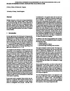
of RN −2 = R2 (since N = 22 = 4). Since mb (x) ≥ 0, mb (y) ≥ 0, and mb (x) + mb (y) ≤ 1 the set B2 of all the possible belief functions on Θ2 is the triangle of Figure 1, whose vertices are the points bΘ = [0, 0]0 , bx = [1, 0]0 , by = [0, 1]0 which correspond respectively to the vacuous belief function bΘ (mbΘ (Θ) = 1), the Bayesian b.f. bx with mbx (x) = 1, and the Bayesian b.f. by with mby (y) = 1. The region P2 of all Bayesian b.f.s on Θ2 is the segment by =[0,1]'
{b(A), A ⊆ Θ, A 6= ∅}, . |Θ| N = 2 , and can then be represented as a point of RN −1 . The belief space associated with Θ is the set of points B of RN −1 which correspond to b.f.s. Let us call . bA = b ∈ B s.t. mb (A) = 1, mb (B) = 0 ∀B 6= A (2) the unique b.f. assigning all the mass to a single subset A of Θ (A-th basis belief function). We proved that (Cuzzolin 2007b), denoting by Eb the list of focal elements of b, Proposition 3. The set of all the belief functions with focal elements in a given collection L is closed and convex in B: {b : Eb ⊆ L} = Cl(bA : A ∈ L), where Cl denotes the convex closure operator: n Cl(b1 , ..., bk ) = b ∈ B : b = α1 b1 + · · · + αk bk , o X αi = 1, αi ≥ 0 ∀i . i
As a consequence, the belief space B is the convex closure of all the basis belief functions bA , B = Cl(bA , ∅ ( A ⊆ Θ). More precisely B is an N − 2-dimensional simplex, i.e. the convex closure of N − 1 (affinely independent (Dubrovin, Novikov, & Fomenko 1986)) points of the Euclidean space RN −1 . The faces of a simplex are all the simplices generated by a subset of its vertices. Each belief function b ∈ B can be written as a convex sum as X b= mb (A)bA . (3) ∅(A⊆Θ
Since a probability is a b.f. assigning non zero masses to singletons only, Proposition 3 implies that the set P of all Bayesian b.f.s is the simplex P = Cl(bx , x ∈ Θ).
3.2
Binary case
As an example let us consider a frame of discernment containing only two elements, Θ2 = {x, y}. In this very simple case each b.f. b : 2Θ2 → [0, 1] is completely determined by its belief values b(x), b(y) as it is always true that b(Θ) = 1, b(∅) = 0 ∀b ∈ B. We can then represent b as the vector [b(x) = mb (x), b(y) = mb (y)]0
P2 COy
B2
b
mb(y)
bΘ=[0,0]'
COx
mb(x)
bx =[1,0]'
Figure 1: The belief space B for a binary frame is a triangle in R2 whose vertices are the basis b.f.s focused on {x}, {y} and Θ, (bx , by , bΘ respectively). The probability region is the segment Cl(bx , by ), while consonant and consistent b.f.s live in the union of two segments CS x = COx = Cl(bΘ , bx ) and CS y = COy = Cl(bΘ , by ). Cl(bx , by ). In the binary case consonant belief functions can have as sets of focal elements one between {{x}, Θ2 } and {{y}, Θ2 }. Therefore the space of co.b.f.s CO2 is the union of two convex components CO2 = COx ∪ COy = Cl(bΘ , bx ) ∪ Cl(bΘ , by ) and coincides with the region CS 2 of consistent b.f.s, as the latter cannot have both {x} and {y} as focal elements.
3.3
The consonant complex
In the general case (Cuzzolin 2004b) the geometry of co.b.f.s can be described by means of the notion of simplicial complex (Dubrovin, Novikov, & Fomenko 1986). Definition 1. A simplicial complex is a collection Σ of simplices which satisfies the following properties: 1. if a simplex belongs to Σ, then all its faces of any dimension belong to Σ; 2. the intersection of any two simplices is a face of both the intersecting simplices. Let us consider for instance two triangles (2-dimensional simplices) in R2 . Roughly speaking, the second condition says that their intersection cannot contain points of their interiors (Figure 2-left) or be an arbitrary subset of their borders (middle), but has to be a face (right, in this case a single vertex). It can be proven that (Cuzzolin 2004b) Proposition 4. The region CO of consonant belief functions in the belief space is a simplicial complex.
Figure 2: Constraints on the intersection of simplices in a complex. Only the right-hand pair meets condition 2. of the definition of simplicial complex. More precisely, CO is a collection of maximal simplices Cl(bA1 , ..., bAn ), each of them associated with a maximal chain of subsets in 2Θ : A1 ⊂ · · · ⊂ An , |Ai | = i. In the binary example COx and COy are the two maximal simplices forming a simplicial complex (as they intersect in a vertex).
4
Let us pick for instance two possible cores C1 = {x, y} and C2 = {x}. The lists of focal elements associated with cs.b.f.s with cores C1 and C2 are respectively Ebx = {A 3 x} = {{x}, {x, y}, {x, z}, Θ} Ebx,y = {A ⊇ {x, y}} = {{x, y}, Θ} ( Ebx which confirms that all maximal lists of f.e.s for consistent b.f.s are associated with singletons of Θ (x in this case). In the ternary case the maximal collections (4) of consistent f.e.s are then {A 3 x}, {A 3 y}, and {A 3 z}. The number of simplicial components is 3, and their dimension |{A 3 x}| − 1 = 3: Cl(bA : A 3 x) = Cl(bx , b{x,y} , b{x,z} , bΘ ), Cl(bA : A 3 y) = Cl(by , b{x,y} , b{y,z} , bΘ ), Cl(bA : A 3 z) = Cl(bz , b{x,z} , b{y,z} , bΘ ). The geometry of consistent belief functions in the ternary frame can then be represented as in Figure 3. The consonant subspace CO3 , for comparison, is the union bz
Geometry of the consistent subspace
As co.b.f.s and cs.b.f.s are associated with possibility measures and distributions respectively, it is natural to conjecture that consistent belief functions may have a similar geometric behavior. All possible lists of f.e.s associated with consistent b.f.s obviously correspond to all possible collections of intersecting events: m \ {A1 , ..., Am ⊆ Θ : Ai 6= ∅}.
b{x,z}
bx
CS3
Geometrically, Proposition 3 implies that all the b.f.s whose focal elements belong to such a collection form the simplex Cl(bA1 , ..., bAm ). This collection is “maximal” when it is not possible to add another event Am+1 such that ∩m+1 i=1 Ai 6= ∅. Collections of events with non-empty intersection are maximal iff they have the form (4)
for some singleton x ∈ Θ. By Proposition 3 the region of cs.b.f.s is the union of a number of simplices, each associated with a maximal collection of the form (4): [ CS = Cl(bA , A 3 x). x∈Θ
The number of such maximal simplices of CS is then obvi. ously the number of singletons, i.e. the cardinality n = |Θ| of Θ. Each of them has |{A : A 3 x}| = |{A ⊆ Θ : A = {x} ∪ B, B ⊂ {x}c }| = c
= 2|{x} | = 2n−1 vertices, so that their dimension as simB plices of B is 2n−1 − 1 = dim (as the dimension of the 2 n whole belief space is dim B = 2 − 2). As bΘ belongs to all maximal simplices CS is connected.
4.1
A ternary example
In the case of a frame of size 3 Θ = {x, y, z} all b.f.s b ∈ B3 are 6-dimensional vectors: [b(x), b(y), b(z), b({x, y}), b({x, z}), b({y, z})]0 .
by b{x,y}
i=1
{A ⊆ Θ : A 3 x}
b {y,z}
bΘ
Figure 3: The consistent CS 3 subspace for Θ = {x, y, z}. of the six simplices Cl(bx , b{x,z} , bΘ ), Cl(bx , b{x,y} , bΘ ), Cl(by , b{x,y} , bΘ ), Cl(by , b{y,z} , bΘ ), Cl(bz , b{y,z} , bΘ ), and Cl(bz , b{x,z} , bΘ ) which are also faces of CS 3 .
4.2
The consistent complex
The region of consistent b.f.s is indeed also a simplicial complex, i.e. a collection of simplices satisfying Definition 1. Theorem 2. CS is a simplicial complex. Proof. Property 1. of Definition 1 is trivially satisfied. As a matter of fact, if a simplex Cl(bA1 , ..., bAn ) corresponds to focal elements with non-empty intersection, clearly points of any face of this simplex (obtained by selecting a subset of vertices) will be b.f.s with non-empty core, and will then correspond to cs.b.f.s. About property 2., consider the intersection of two maximal simplices of CS associated with two distinct cores C1 , C2 ⊂ Θ: Cl(bA : A ⊇ C1 ) ∩ Cl(bA : A ⊇ C2 ). Now, each convex closure of points b1 , ..., bm in a Cartesian space is included in the affine space they generate: . m) = n Cl(b1 , ..., bm ) ( a(b1 , ..., bX o . = b : b = α1 b1 + · · · + αm bm , αi = 1 i
(since this just means that we relax the positivity constraint on the coefficients αi ). But the basis b.f.s {bA : ∅ ( A ( Θ} are linearly independent (as it is straightforward to check), so that a(bA , A ∈ L1 ) ∩ a(bA , A ∈ L2 ) 6= ∅ ⇔ L1 ∩ L2 6= ∅ where L1 , L2 are lists of subsets of Θ. Here L1 = {A ⊆ Θ : A ⊇ C1 }, L2 = {A ⊆ Θ : A ⊇ C2 }, so that the condition is {A ⊆ Θ : A ⊇ C1 } ∩ {A ⊆ Θ : A ⊇ C2 } = = {A ⊆ Θ : A ⊇ C1 ∪ C2 } 6= ∅. As C1 ∪ C2 ⊇ C1 , C2 we have that Cl(bA , A ⊇ C1 ∪ C2 ) is a face of both simplices.
5
The twin geometry of consistency and combinability
The geometric approach to the theory of evidence can be applied in particular to possibility theory by analyzing the geometry of consonant and consistent belief functions. Some sort of duality seems to appear, as the geometric counterparts of belief measures are simplices, while the geometric loci of possibility measures and assignments are simplicial complexes (see Figure 4-left). A similar duality appears when considering the relationship
belief measures, probability measures
conditional subspace
the class of belief functions on Θ which are not combinable with each and every other b.f. (singular subspace). The singular subspace is itself a simplicial complex: The duality between combinable/non-combinable b.f.s is again reflected in the dichotomy simplex-complex (Figure 4-right). This is related to the fact that cs.b.f.s can be constructed from non-combinable b.f.s, and vice-versa. B.F.s in Sing are characterized by the property that the union of their focal elements is a proper subset of Θ: [ b ∈ Sing ⇔ Ai Θ, Ai ∈Eb
where Eb denotes again the list of focal elements of b. Equivalently, there exists a non-empty subset of Θ which has empty intersections with each f.e. of b. Any b.f. b0 with focal elements in this subset will not be combinable with b. We can then write [ Ai ⊆ {x}c b ∈ Sing ⇔ Ai ∈Eb
for some element x ∈ Θ. By Proposition 3, b.f.s with focal elements in the list L = {A ⊆ {x}c } form the simplex Cl(bA : A ⊆ {x}c ). As there are n of such subsets (one for each singleton) the region of “singular” b.f.s is [ Sing = Cl(bA : A ⊆ {x}c ). (5) x∈Θ
Theorem 3. Sing (5) is a simplicial complex.
possibility measures, assignments
singular subspace
Proof. As a matter of fact, following the same line of the proof of Theorem 2, each pair of simplices in the collection (5) has a common intersection Cl(bA : A ⊆ {x}c ) ∩ Cl(bA : A ⊆ {y}c ) = = Cl(bA : A ⊆ {x, y}c )
Figure 4: A pictorial representation of geometric dualities between notions of uncertainty theory. between the notion of consistency and that of combinability in Dempster’s theory. Definition 2. The orthogonal sum or Dempster’s sum of two b.f.s b1 , b2 on Θ is a new belief function b1 ⊕ b2 on Θ with b.p.a. P mb (B) mb2 (C) mb1 ⊕b2 (A) = PB∩C=A 1 B∩C6=∅ mb1 (B) mb2 (C) where mbi denotes the b.p.a. associated with bi . When the denominator of the above equation is nil the two functions are said to be non-combinable. Now, we have seen (Cuzzolin 2004a) that the conditional subspace . hbi = {b ⊕ b0 , ∀b0 ∈ B : ∃b ⊕ b0 } obtained by combining through Dempster’s rule a given b.f. b with all other b.f.s on the same frame (if such a combination exists) is a simplex. Let us focus here on noncombinable belief functions, and call . Sing = {b ∈ B : ∃b0 ∈ B :6 ∃b ⊕ b0 }
which is a face of both (Property 2 of Definition 1). Besides, their faces correspond to b.f.s whose union of focal elements is obviously a proper subset of Θ (having less focal elements), and then belong to Sing (Property 1). Figure 5 shows the singular complex for a ternary frame, and its relationship with CO3 (CS 3 is not shown for sake of simplicity). Examining Figures 5 and 3 we can see that each . maximal component Singx = Cl(bA : A ⊆ {x}c , A 6= ∅) of Sing corresponds to a component CS x of CS: Singx = Cl(bA : ∅ ( A ⊂ {x}c ) l CS x = Cl(bA : A 3 x) = Cl(bx , bA : A ) {x}) = = Cl(bx , Cl(bA : A = B ∪ {x}, ∅ ( B ⊂ {x}c )).
(6)
The interpretation is straightforward: each consistent b.f. is obtained by a singular b.f. by adding to each of its f.e.s a subset of Θ \ ∪i Ai , Ai ∈ Eb . In fact, each maximal simplex Singx of the singular complex is nothing but a replica of the belief space B{x}c for the frame {x}c : for instance, in the above ternary example the triangle Cl(bx , by , b{x,y} ) is isomorphic to the binary belief space B2 (see Figure 1).
Sing y
b{x,z}
by =[0,1]'
bz b{y,z}
P3
m b(y)
bx
Sing x
y
b
m b(y) + m b(Θ) 2
by
CS y
b{x,y}
CO3
b
m b(y)
b
Sing z
bΘ=[0,0]'
m b(x)
CS x
Figure 5: The singular subspace for a ternary frame, and the related consonant subspace. Each maximal component Singx of Sing is isomorphic to the belief space B2 = Cl(by , bz , b{y,z} ) for the binary frame ({x}c = {y, z}).
Figure 6: A belief function b as convex combination of its consistent coordinates in the binary belief space. pignistic probability associated with b: . X m(A) BetP [b](x) = . |A|
6 A decomposition in consistent components A natural application of the geometric approach is the problem of finding approximations of belief functions belonging a given class of measures. We then close this paper by pointing out an interesting decomposition (closely related to the pignistic transformation (Smets & Kennes 1994)) of any belief function b into consistent components, which be interpreted as the natural projections of b on the maximal components of the consistent simplicial complex. Let us then consider again the binary case. As a matter of fact, any b.f. b ∈ B2 b = mb (x)bx + mb (y)by + mb (Θ)bΘ can be written as theà following combination (Figure! 6) ³ ´ m(Θ) m(x) 2 b = m(x) + m(Θ) + m(Θ) bx + m(Θ) bΘ 2 m(x)+ 2 m(x)+ 2 à ! ³ ´ m(Θ) m(y) 2 + m(y)+ m(Θ) , which m(Θ) )by + m(Θ) bΘ 2 2
m(y)+
by =
A3x
In other words, any b.f. b ∈ B2 can be written as a convex combination of two consistent belief functions b = BetP [b](x)bx + BetP [b](y)by bx ∈ CS x and by ∈ CS y , whose coefficients are the values of the pignistic function. In the general case, the consistent belief functions . bx =
m(Θ) 2 bΘ , m(x) + 2 m(x) + m(Θ) 2 m(Θ) m(y) 2 )b + b . y m(Θ) Θ m(y) + m(Θ) m(y) + 2 2
m(x)
b + m(Θ) x
Now, we can notice that m(x) + m(Θ) = BetP [b](x) and 2 m(Θ) m(y) + 2 = BetP [b](y), where BetP [b] denotes the
X m(A) 1 bA , BetP [b](x) |A|
x∈Θ
A3x
can be considered as “consistent projections” of b onto the maximal components CS x , x ∈ Θ of the consistent subspace. As a matter of fact we can write
2
is convex, as (mb (x) + mb (Θ)/2) + (mb (y) + mb (Θ)/2) = mb (x) + mb (y) + mb (Θ) = 1 and mb (x) + mb (Θ)/2 ≥ 0, mb (y) + mb (Θ)/2 ≥ 0. In fact, this is the only way each belief function b ∈ B2 can be consistently decomposed as a convex combination of two points of CS x , CS y : bx =
bx =[1,0]'
m b(x)
m b(x) + m b(Θ) 2
bΘ
m(y)+
x
b=
X
m(A)bA =
A⊆Θ
=
X x∈Θ
BetP [b](x)
X X m(A) bA = |A|
x∈Θ A3x m(A) A3x |A| bA
P
BetP [b](x)
=
X x∈Θ
BetP [b](x)bx .
(7) According to Equation (7), each b.f. b lives in the n − 1 . dimensional simplex P b = Cl(bx , x ∈ Θ) (see Figure 7) and its convex coordinates in P b (“consistent” coordinates) coincide with the coordinates of the pignistic probability in the probability simplex P. This argument in a sense mirrors another well known result which states that a belief function is a convex sum of a probability measure and a possibility measure. This is clear from Figure 1, where the reader can easily appreciate that b lies on a manifold of segments joining COx (COy ) and P.
bx
P CSx
bz
x
b BetP[b]
P y
by
CSy
b
b
b
z
b
bΘ
CSz
Figure 7: Pictorial representation of the role of the pignistic values BetP [b](x) for a belief function and the related pignistic function. Both b and BetP [b] live in a simplex (respectively P = Cl(bx , x ∈ Θ) and P b = Cl(bx , x ∈ Θ)) on which they possess the same convex coordinates. The vertices bx , x ∈ Θ of the simplex P b can be interpreted as consistent projections of the belief function b on the simplicial complex of consistent belief functions CS.
6.1
Consistent coordinates and inner approximations
Equation (7) draws a connection between the notions of belief, probability, and possibility as it relates each belief function to its “natural” probabilistic (the pignistic function) and consistent (the quantities bx ) proxy. It remains to understand whether those functions bx can be interpreted as some sort of consistent approximations of b, i.e. the cs.b.f.s which minimize some sort of distance between b and the consistent subspace. As a matter of fact, consistent belief functions can be easily approximated in terms of possibility measures or consonant belief functions. Inner consonant approximations (Dubois & Prade 1990) of a b.f. b are those co.b.f.s such that c(A) ≥ b(A) ∀A ⊆ Θ (or equivalently plc (A) ≤ plb (A) ∀A). Such an approximation exists indeed iff b is consistent. In the binary case this means that inner approximations of b exist iff b is already consonant: b ∈ COx or b ∈ COy . The optimal inner approximation is the co.b.f. cˆ such that plcˆ(x) = plb (x) ∀xinΘ. It is rather interesting to wonder what are the relationships between the consistent coordinates obtained above and Dubois and Prade’s inner approximations: We are going to investigate this issue in the near future (Cuzzolin 2007c).
7 Comments In this paper we completed the analysis of the geometry of finite possibility measures by focusing on consistent belief functions, in virtue of their relationships with possibility assignments, on one side, and singular belief functions on the
other. On a wider perspective, this study places a new element in the geometric semantics of the theory of evidence. As belief functions are points of a simplex, possibility measures form a simplicial complex, and Dempster’s rule itself is nothing but an intersection of linear spaces (Cuzzolin 2004a), the Dempster-Shafer formalism can be in fact seen as some form of geometric calculus. The full potential of the geometric approach can be appreciated though in the approximation problem: in the near future we will develop the preliminary results of (Cuzzolin 2004b) and Section 6 into a complete description of the consonant and consistent approximation problems by geometric methods, and relate them to inner and outer approximations (Dubois & Prade 1990). The natural evolution of the belief space formalism is possibly the confluence with the field of geometric probability or continuous combinatorics (Klain & Rota 1997), which studies invariant measures on sets of geometric objects and relates them to additive probability measures. Belief functions ncan be indeed seen as iso-volumes of a convex body in R2 −1 , i.e. the vector of the volumes of all its orthogonal projections onto the space spanned by a subset of the reference axes.
References Baroni, P. 2004. Extending consonant approximations to capacities. In Proceedings of IPMU, 1127–1134. Barthelemy, J. 2000. Monotone functions on finite lattices: an ordinal approach to capacities, belief and necessity functions. In Fodor, J.; Baets, B. D.; and Perny, P., eds., Preferences and Decisions under Incomplete Knowledge. 195–208. Berger. 1990. Robust Bayesian analysis: Sensitivity to the prior. Journal of Statistical Planning and Inference 25:303–328. Caro, L., and Nadjar, A. B. 1999. Generalization of the Dempster-Shafer theory: A fuzzy-valued measure. IEEE Transactions on Fuzzy Systems 7:255–270. Cozman, F. G. 1999. Calculation of posterior bounds given convex sets of prior probability measures and likelihood functions. Journal of Computational and Graphical Statistics 8(4):824–838. Cuzzolin, F. 2004a. Geometry of Dempster’s rule of combination. IEEE Transactions on Systems, Man and Cybernetics part B 34:2:961–977. Cuzzolin, F. 2004b. Simplicial complexes of finite fuzzy sets. In Proceedings of the 10th International Conference on Information Processing and Management of Uncertainty IPMU’04, Perugia, Italy, 1733–1740. Cuzzolin, F. 2007a. Dual properties of relative belief of singletons. submitted to the IEEE Transactions on Fuzzy Systems. Cuzzolin, F. 2007b. A geometric approach to the theory of evidence. IEEE Transactions on Systems, Man and Cybernetics part C, to appear. Cuzzolin, F. 2007c. Metric consistent approximations of belief functions. (in preparation).
Cuzzolin, F. 2007d. Moebius inverses of plausibility and commonality functions and their geometric interpretation. submitted to the International Journal of Uncertainty, Fuzziness, and Knowledge-Based Systems. Cuzzolin, F. 2007e. Two new Bayesian approximations of belief functions based on convex geometry. IEEE Transactions on Systems, Man and Cybernetics part B 37(4). Dempster, A. P. 1968. Upper and lower probabilities generated by a random closed interval. Annals of Mathematical Statistics 39:957–966. Dubois, D., and Prade, H. 1988. Possibility theory. New York: Plenum Press. Dubois, D., and Prade, H. 1990. Consonant approximations of belief functions. International Journal of Approximate Reasoning 4:419–449. Dubrovin, B. A.; Novikov, S. P.; and Fomenko, A. T. 1986. Sovremennaja geometrija. Metody i prilozenija. Moscow: Nauka. Fagin, R., and Halpern, J. 1988. Uncertainty, belief and probability. In Proc. Intl. Joint Conf. in AI (IJCAI-89), 1161–1167. Heilpern, S. 1997. Representation and application of fuzzy numbers. Fuzzy Sets and Systems 91:259–268. Joslyn, C., and Klir, G. 1992. Minimal information loss possibilistic approximations of random sets. In Bezdek, J., ed., Proc. 1992 FUZZ-IEEE Conference, 1081–1088. Joslyn, C. 1991. Towards an empirical semantics of possibility through maximum uncertainty. In Lowen, R., and Roubens, M., eds., Proc. IFSA 1991, volume A, 86–89. Klain, D. A., and Rota, G.-C. 1997. Introduction to Geometric Probability. Cambridge University Press. Klir, G. J.; Zhenyuan, W.; and Harmanec, D. 1997. Constructing fuzzy measures in expert systems. Fuzzy Sets and Systems 92:251–264. Melkonyan, T., and Chambers, R. 2006. Degree of imprecision: Geometric and algebraic approaches. forthcoming in the International Journal of Approximate Reasoning. Nguyen, H. T., and Wang, T. 1997. Belief functions and random sets. In Applications and Theory of Random Sets, The IMA Volumes in Mathematics and its Applications, Vol. 97. Springer. 243–255. Roemer, C., and Kandel, A. 1995. Applicability analysis of fuzzy inference by means of generalized Dempster-Shafer theory. IEEE Transactions on Fuzzy Systems 3:4:448–453. Seidenfeld, T., and Wasserman, L. 1993. Dilation for convex sets of probabilities. Annals of Statistics 21:1139– 1154. Shafer, G. 1976. A Mathematical Theory of Evidence. Princeton University Press. Smets, P., and Kennes, R. 1994. The Transferable Belief Model. Artificial Intelligence 66:191–234. Smets, P. 1990. The transferable belief model and possibility theory. In Y., K., ed., Proceedings of NAFIPS-90, 215–218.
Yager, R. R. 1999. Class of fuzzy measures generated from a Dempster-Shafer belief structure. International Journal of Intelligent Systems 14:1239–1247. Yao, Y. Y., and Lingras, P. J. 1998. Interpretations of belief functions in the theory of rough sets. Information Sciences 104(1-2):81–106.