house 1 has About 500 of product 1' or even more abstract. 'Warehouse 1's stock ..... burgh (W3) and 6 customers in Plymouth (C1), Cardiff (C2),. Derby (C3) ...
An Interval Type-2 Fuzzy Distribution Network Simon M. Miller, Viara Popova, Robert John, Mario Gongora Centre for Computational Intelligence, De Montfort University, Leicester, UK.
Email: {smiller,vpopova,rij,mgongora}@dmu.ac.uk Abstract— Planning resources for a supply chain is a major factor determining its success or failure. In this paper we introduce an Interval Type-2 Fuzzy Logic model of a distribution network. It is believed that the additional degree of uncertainty provided by Interval Type-2 Fuzzy Logic will allow for better representation of the uncertainty and vagueness present in resource planning models. First, the subject of Supply Chain Management is introduced, then some background is given on related work using Type-1 Fuzzy Logic. A description of the Interval Type-2 Fuzzy model is given, and a test scenario detailed. A Genetic Algorithm uses the model to search for a near-optimal plan for the scenario. A discussion of the results follows, along with conclusions and details of intended further work. Keywords— Distribution model, Evolutionary Computing, Interval Type-2 Fuzzy Logic, Resource Planning, Supply Chain Management
1
Introduction
There are a number of definitions of Supply Chain Management (SCM), each having minor variances but describing the same core idea. SCM is the management of material flow in and between facilities including vendors, manufacturing/assembly plants and distribution centres [1]. Planning the allocation of resources within a Supply Chain (SC) has been critical to the success of manufacturers, warehouses and retailers for many years. Mastering the flow of materials from their creation to the point of sale offers considerable advantages to those within a well managed SC. Poorly managed resources result in two main problems: stock outs and surplus stock. The consequence of stock outs is lost sales, and potentially lost customers. Surplus stock causes additional holding cost and the possibility of stock losing value as it becomes obsolete. Holding some surplus stock is advantageous however; safety stock can be used in the event of an unexpected increase in demand or to cover lost productivity. The problem has been addressed numerous times in the literature using different approaches. An overview of traditional and Computational Intelligence approaches to supply-chain resource planning can be found in [2]. Here a novel approach using Type-2 Fuzzy Logic (T2FL) [3] is reported together with optimisation by means of a Genetic Algorithm (GA)[4]. This research is part of a project on demand forecasting and resource planning (Data Storage, Management, Retrieval and Analysis: Improving Customer Demand and Cost Forecasting Methods funded by the Technology Strategy Board in the UK). The project aims to: (1) improve the forecasting of demand by using a variety of disparate sources and statistical and Machine Learning (ML) methods for analysis; (2) improve the allocation of resources in which the generated forecast is used as an input and the output is a (long- or short-term) plan of raw materials and resources within the supply chain in order to
meet such demand. Various degrees of uncertainty are present in the different data sources used that are amplified in the generated forecast by applying methods of analysis with (again) varying degrees of inherent uncertainty. Furthermore, other data that is often used in resource planning such as transportation and other costs, customer satisfaction information, etc. is also uncertain. Therefore, FL and especially T2FL are particularly appropriate for this problem. While Type-1 FL (T1FL) has successfully been used many times for modelling SC operation (see Section 2), T2FL has been shown to offer a better representation of uncertainty on a number of problems (e.g., [5] and [6]). However, to date T2FL has not been applied to SCM in the literature. This paper presents a T2FL model of a SC problem which is optimised by a GA to find a near-optimal configuration. The paper is organised as follows. Section 2 discusses Fuzzy Logic and its application to SCM. Section 3 introduces the model and the test case used for evaluation. The results from the experiments on the test case are presented in Section 4. Section 5 concludes the paper with a summary and future research directions.
2
Fuzzy Logic for Supply Chain Management
FL and GAs have been successfully used for supply chain modelling [2] and are particularly appropriate for this problem due to their capacity to tackle the inherent vagueness, uncertainty and incompleteness of the data used. A GA [4] is a heuristics search technique inspired by evolutionary biology. Selection, crossover and mutation are applied to a population of individuals representing solutions in order to find a nearoptimal solution. FL is based on fuzzy set theory and provides methods for modelling and reasoning under uncertainty, a characteristic present in many problems, which makes FL a valuable approach. It allows data to be represented in intuitive linguistic categories instead of using precise (crisp) numbers which might not be known, necessary or in general may be too restrictive. For example, statements such as ‘the cost is about n’, ‘the speed is high’ and ‘the book is very old’ can be described. These categories are represented by means of a membership function which defines the degree to which a crisp number belongs to the category. In this research the aim is to allow linguistic terms to be used by Supply Chain Managers when describing their operation. For example, instead of asking for crisp numbers to describe the current stock level of a product, we may allow them to make statements like ‘Warehouse 1 has About 500 of product 1’ or even more abstract ‘Warehouse 1’s stock level of product 1 is low’. By removing the need for exact information it is possible to produce a system that is much more usable when the information available is vague, uncertain or incomplete.
T1FL has been applied to SC modelling numerous times with good results. Some of the research that is considered most relevant for this paper is discussed in the following paragraphs. Petrovic et al. [7] use fuzzy sets to model vagueness and imprecision in customer demand, external supplier reliability and supply within a SC. The system demonstrates the effect of differing conditions and strategies on fill rate and holding costs of a SC. The results of the evaluation show that there is a slight improvement in the performance of the SC when the inventories are partially co-ordinated. In [8] Petrovic et al. employ two-level fuzzy optimisation to find ideal order-up-to quantities in a one warehouse-multiple retailer SC. The problem is decomposed for individual control of the warehouse and retailers; a co-ordination mechanism provides overall control of the SC. Customer demand, inventory levels, holding cost, and shortage cost are represented by fuzzy sets. A measure of satisfaction is derived from the cost incurred at each element. The solution produced by the system is the best compromise between members, though not necessarily the cheapest. In [9] a fuzzy system is used with a GA to model a SC. The model uses a global policy of management with emphasis on integrating the production and distribution models. The GA searches for a near-optimal configuration; fuzzy sets are used to describe costs, returns, production capacities, storage capacities and forecasts. The proposed fuzzy method, a crisp method and a non-integrated method are compared. The crisp system is unable to produce a feasible configuration if actual demand is lower than the forecast. In contrast, the fuzzy model presented is robust and able to cope with fluctuation in demand and production capacity with little impact on profitability. The non-integrated model performed significantly worse than the fuzzy integrated model. A similar approach is presented by Wang and Shu [10]. FL is used to represent customer demand, processing time and delivery reliability; a GA finds order-up-to levels. The system attempts to find the configuration that incurs the minimum cost. An optimism-pessimism index is set by the user and passed to the system. When optimistic, the model assumes the best case scenario for material response time. A pessimistic attitude produces the opposite effect. The results show that more pessimistic strategies increase the fill rate, reducing the sales lost through stock outs, and incur higher inventory cost as more stock is kept. More optimistic strategies result in a drop in fill rate and an increase in sales loss, though inventory cost is also reduced. T2FL [3] provides the means to model an additional dimension of uncertainty as the membership functions are themselves modelled as fuzzy numbers, thus providing the means for a more accurate representation of uncertainty in a complex system and the potential for better performance. On a number of problems, T2FL has been shown to outperform T1FL (e.g., [5] and [6]), however it has not yet been applied to SC modelling in the literature. In this paper, Interval Type-2 FL (IT2FL) [11] is used which is computationally cheaper as it restricts the additional dimension, referred to as secondary membership function, to only take the values 0 or 1. We believe that the extra degree of freedom will allow a better representation of the uncertain and vague nature of data used in SCM. Section 3 describes the created model in detail as well
as the test case used for evaluation.
3 Model The model presented here describes a distribution network consisting of a set of manufacturing warehouses and customers. Each warehouse holds one or more products; when demand of an item is forecast for a customer, a warehouse is selected to satisfy the demand. Before the model is used it is configured to model the required network. This is done by telling the model how many warehouses, customers and products there are, the distances between the warehouses and customers, the costs associated with network operation and how many periods the model is to run for. As input, the model takes a forecast of demand over a given period and a suggested resource plan for the warehouses detailing how much of each item to hold at each warehouse in each period. The purpose of the model is to calculate the cost of a given resource plan. This is calculated based on a number of factors: Production Cost - Each product is assigned an individual production cost. The total production cost for each batch is calculated by multiplying the number of items by their production cost. Holding Cost - A holding cost is charged if a product is kept in a warehouse for more than one period. The cost is calculated by taking a specified percentage of the purchase price of the goods held, for items carried over from one period to the next. The purpose of the charge is to represent the costs of storing items, depreciating value of stock and the losses incurred by tying up capital in unsold stock. Transport Cost - The cost of transporting goods is produced using a matrix of distances between warehouses and customers, and a list of transport costs per mile for each product. The product of the relevant cost and mileage gives the overall transport cost for a batch of product. Stock out cost - Stock out is the shortfall of a product in a particular period. In this model we make the assumption that the customer is always provided with an item. If it is not in the warehouse, it is purchased at full retail price from a competing producer. The stock out cost is the sum of the value of items that had to be purchased in this period. Cost of purchase is not the only penalty incurred when stock out occurs. The customer may cancel their order if they discover that it is not in stock, and will be ordered elsewhere. To represent this a multiplier is applied to the stock out cost, taking into account the cost of lost orders. Batch cost - The cost of setting up an order is called the batch cost. This represents the cost of administration and setting up any machines that are required, and picking the items for dispatch. There is a flat fee for each batch which is charged once at each warehouse for the production of a particular item for a particular customer. Using these costs a total cost is produced, allowing comparison of competing solutions. 3.1 Interval Type 2 Fuzzy Logic For the experimental model IT2FL has been used to represent some of the values within the model. Previous examples (as
discussed in Section 2) of research in this area have focused on the use of T1FL; we believe there exists an opportunity to exploit the extra degree of uncertainty provided by IT2FL in a model of this type. As the model operates on fuzzy numbers, fuzzy arithmetic is used to calculate costs. This involves taking fuzzy sets, discretising them, performing the arithmetic operation, and then reconstructing the fuzzy set. In this model, fuzzy sets are represented using a series of α-cuts. Each set is an array of pairs of intervals. Each pair shows the area of values covered at a particular value of µ, the first interval is the left hand side of the set, and the second the right. Storing the sets in this way removes the need to discretise before fuzzy arithmetic is performed, and then reconstruct the result. Operations on fuzzy sets are performed at interval level, corresponding intervals (at the same µ) are taken from two sets, the operation performed and the result stored in a third fuzzy set. The following values are represented by IT2 fuzzy numbers: forecast demand, inventory level, transportation distances, transportation cost, stock out level, stock out cost, carry over and holding cost. For each of these values we can use the linguistic term ‘about n’, e.g., forecast demand of product 1 for customer 1 in period 1 may be ‘about 200’. When the fuzzy total cost for a solution has been calculated, it is defuzzified to produce a crisp cost value. Fig. 1 shows how the set ‘about 200’ may look with the α-cut representation used, where x is the scale of values being represented. The set is described using a collection of pairs of intervals. Each pairing represents the left and right hand intervals of the set for a given value of µ. As stated before, representing the set in this way considerably simplifies the arithmetic operators that are applied as simple interval arithmetic is used throughout, without discretisation or reconstruction. 1 0.8 0.6 µ 0.4
For M αi we take the mid-point between the current and subsequent α-cut’s µ values. The mid-point values are used along with the height (H) and length (L) to calculate the weighted area of each pair of intervals, giving more weight the those with higher µ values. n−1 X
Mix Hi Li M αi
i=0 n−1 X
(1) Hi L i M
αi
i=0
where:
Mix =
α
α
xl i +xl i 2 1 2
for left interval (2)
α
α
xr2i +xr1i 2
for right interval
Hi = αi+1 − αi
Li =
αi α xl2 − xl1i
i xα r2
−
i xα r1
(3)
for left interval (4) for right interval
αi + αi+1 (5) 2 In the test scenario, µ is discretised in a uniform manner. This removes the need to calculate the height of intervals as they are all the same, and therefore cancel out. The process used in the actual code is given in (6). M αi =
n−1 X
Mix Li M αi
i=0 n−1 X
(6) Li M
αi
i=0
It should be pointed out that while this method works well for the convex fuzzy numbers used in this system, it cannot be applied to non-convex fuzzy sets as the interval representation employed will cease to accurately represent the set. In 198 199 200 201 202 203 this model, the fuzzy numbers will always be convex. In addix tion to this the method of representation being used ensures that the intervals are already present, no further discretisaFigure 1: Interval representation of IT2 fuzzy set ‘about 200’ tion is required. Using a method that requires re-discretisation would incur unnecessary computation. A consideration for future work is the possibility of using another approach such as 3.2 Defuzzification the one proposed by Karnik and Mendel [12], however this The defuzzification process used is described in (1) where n method would involve rediscretising on the x axis, at present is equal to the number of α-cuts, and l and r denote the left the model is discretised on the µ axis. and right hand intervals respectively. To reference the left and right endpoints of the intervals 1 and 2 are used; so l1 refers 3.3 Optimisation to the left bound of l and l2 the right bound. M denotes the The focus of the experiment described here is the validation mid-point of an interval, in the case of Mix this means the cen- of an IT2FL model that has been constructed. This is to be tres of the intervals in x described by the ith pair of intervals. achieved by using the model to find a good resource plan for a 0.2
given forecast, confirming that the model can be used to evaluate potential solutions. A GA has been chosen for this purpose. GAs have been used successfully in previous work (e.g., [13] and [14]) to find good solutions with T1FL models. GAs are useful when a search area is too large to allow evaluation of every solution. In this case the GA is used to search for a resource plan that incurs the minimum cost. The GA has a population of 250 and is executed for 500 generations, in all 125000 solutions are evaluated. Even in this relatively small problem the GA only covers approximately 10162 of the total search space. New generations consist of: 1% individuals produced with elitism, 20% copied individuals, 20% individuals created with single point crossover and 59% of individuals created using mutation. A description of the chromosome, operators and processes employed follows. Chromosome - The chromosome used to describe potential solutions is a 3-D matrix of inventory levels. Columns represent customers, and rows represent a product at a warehouse. If there are 3 warehouses and 5 products this will result in 15 rows. The first 5 rows will be products 1 to 5 for warehouse 1, and second 5 for warehouse 2 and so on. The third dimension represents the period, in each period there is a complete inventory plan for all warehouses and customers. Initial population - The initial population is randomly generated. Each element of the resource plan matrix can be a number between 0 and 500 in steps of 100. This has been done to reflect the fact that in industry, products are usually manufactured in round quantities. If the model suggests that a warehouse should make 102 of product 1, this could lead to difficulties and extra expense. Limiting the valid inventory numbers also has the side effect of reducing the search space.
products we would have 20 rows; in this case the first 10 rows of the first parent and the final 10 of the second parent would be used to create a new individual. If the example were to span 6 periods, we would take the first 10 rows for all 6 periods of the first parent, and the final 10 rows for all 6 periods from the second to create our new individual. Mutation - To create a mutated individual, a parent is selected, then one of the elements of its resource plan is randomly replaced with another valid value to create a new child. 3.4 Test Scenario The test scenario is as follows: The distribution network consists of 3 manufacturing warehouses located in Bristol (W1), Manchester (W2) and Edinburgh (W3) and 6 customers in Plymouth (C1), Cardiff (C2), Derby (C3), Liverpool (C4), Newcastle (C5) and Aberdeen (C6). Each manufacturing warehouse holds the same 5 products, and may supply any customer. The model will be executed over one period and holding costs are 10% of the purchase price of an item per period. Stock outs will be charged at 5 times the cost of purchasing an item, per item short. Each batch of product produced will incur a batch cost of £100. Table 1 details the costs associated with each product. Table 1: Product costs (£s) Product 1 2 Purchase price (per item) 3 4 Production cost (per item) 2 3 Transport cost (per item/per mile) 1 2
3 2 1 1
4 3 2 3
5 3 2 1
The forecast being used states that each customer would like 200 of each product. The location of the manufacturing warehouses and customers have been arranged so that a good solution is easily identifiable. Each warehouse has 2 customers that are best served by it. Table 2 shows how an ideal plan should look. In this case the problem is intentionally kept relatively simple, making it easy to evaluate the found solution and see if it is near the optimal solution. Clearly, simple problems do not require such a system in order to solve them. The work shown here is an initial experiment, future work will build upon this so that it can be applied to larger non-trivial Selection - Selection is performed using a fitness ranking problems where the benefit from the system will be greater. The next section presents and interprets the results from the proportionate method similar to roulette wheel selection. First experiments with the GA. all solutions in the population are ranked by fitness. They are then given a number of elements of an array in proportion to 4 Results their fitness ranking. For example, if we have a population of 250 the fittest individual would be allocated 250 elements As stated previously, in each test the GA was applied to the in the array, the second fittest 249 and so on. An element model using 250 individuals over 500 generations. The test of the array is then selected at random, and the identification was repeated 10 times with differing random seeds, the best number of the individual it contains is used to retrieve a parent. solution found in each test was recorded. Table 3 shows the This tombola style approach ensures that it is possible for any costs incurred by the best solution found in each test. For refindividual to be selected, while weighting in favour of those erence, the cost of the ideal solution presented is £19178.26. with greater fitness. Using the IT2FL model the GA is able to find solutions Crossover - Crossover is achieved with a single point that are close to the optimum. The best solution found is crossover. Two parents are selected using the method of se- just £264.76 (1.38%) from the ideal solution, and the mean lection described. Then, a new individual is created with the difference between solutions found and the ideal solution is first half of the first parent and the second half of the second £1344.79 (7.01%). Table 4 shows the best solution found parent. Division is done by rows, if we have 5 nodes with 4 (with random seed 1). Comparing this solution with the ideal Fitness evaluation - Fitness is evaluated using the IT2FL model described. Candidate solutions are given to the model which evaluates them, and returns the cost. The cheaper a solution is, the fitter it is judged to be. In reality, cost may not be the only factor in deciding how much of a product to stock at each warehouse. Other criteria such as customer service level can also be used to prevent the system from choosing solutions that do not meet service requirements. Customer service level could be calculated by looking at the percentage of orders fulfilled completely, or orders fulfilled on time.
Prod. 1 2 3 4 5 1 2 3 4 5 1 2 3 4 5
Table 2: Ideal solution C1 C2 C3 C4 200 200 0 0 200 200 0 0 200 200 0 0 200 200 0 0 200 200 0 0 0 0 200 200 0 0 200 200 0 0 200 200 0 0 200 200 0 0 200 200 0 0 0 0 0 0 0 0 0 0 0 0 0 0 0 0 0 0 0 0
C5 0 0 0 0 0 0 0 0 0 0 200 200 200 200 200
Table 4: Solution found with a random seed of 1 Ware. Prod. C1 C2 C3 C4 C5 C6 W1 1 200 200 0 200 0 0 W1 2 200 200 0 0 0 0 W1 3 200 200 0 0 0 0 W1 4 200 200 0 0 0 0 W1 5 200 200 0 0 0 0 W2 1 0 0 200 0 200 0 W2 2 0 0 200 200 0 0 W2 3 0 0 200 200 200 0 W2 4 0 0 200 200 0 0 W2 5 0 0 200 200 200 0 W3 1 0 0 0 0 0 200 W3 2 0 0 0 0 200 200 W3 3 0 0 0 0 0 200 W3 4 0 0 0 0 200 200 W3 5 0 0 0 0 0 200
C6 0 0 0 0 0 0 0 0 0 0 200 200 200 200 200
Table 3: Results of test - Best fitness Seed Best Fitness (£s) 0 19789.32 1 19443.02 2 20860.01 3 21048.27 4 20407.71 5 20854.52 6 20952.15 7 20950.17 8 20229.67 9 20695.66
90000 80000 Cost of best solution found (£s)
Ware. W1 W1 W1 W1 W1 W2 W2 W2 W2 W2 W3 W3 W3 W3 W3
70000 60000 50000 40000 30000 20000 10000 0
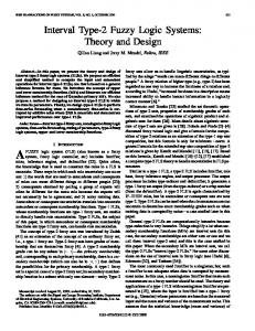
solution we can see that not only are the plans found costeffective, but also represent a sensible allocation of resources. The found solution is very close to the ideal solution, and where there are differences the found model is producing the correct amount of product, but a different warehouse has been chosen. This would not be the case if the model was inadequate for the problem and did not provide a clear distinction between good and bad solutions. All customers will receive their order, the only negative point is that some of customer 4 and 5’s orders could be supplied by a closer warehouse. When the program begins, the best individual in the first generation tends to cost around £70000. Fig. 2 shows a typical run, in this case for the test with a random seed of 1. Evolution can clearly be seen to be heading toward the ideal solution, we also know what the perfect solution looks like, and that the solutions found are close to it. This suggests that the model is working correctly. If the model were not correct, evolution may occur, but possibly in an unexpected direction. This could result in cheap solutions that are not sensible, or in an inability to find cost-effective solutions at all. Out of interest, an extra test was run to see whether the GA would find a better solution if it were left to run over more generations. The best seed from the previous tests (random seed 1) was used as a starting point, and the GA was allowed to run for 2500 generations. In generation 2141 the ideal solution was found, proving that using only feedback from the model, the GA is able to find the ideal solution.
0
50
100
150
200 250 300 350 Number of generations
400
450
500
Figure 2: Evolution of best fitness
5
Conclusion
In this paper we have presented an IT2FL model that can be used to model a distribution network. The advantage of this model is that IT2FL accounts for the uncertain nature of the real world, allowing inputs to the model to be vague. IT2FL has been chosen as it is believed that the extra level of uncertainty over T1FL offered will benefit a model of this type, while avoiding the computational complexity of a Generalised Type-2 FL model. Using the model, it was shown that a GA was able to find good resource plans that were both cost-effective and sensible. Over a longer duration, the GA was able to find the ideal solution. As a GA is solely guided by fitness and essentially ‘blind’ to the practicality of the solutions it finds, this was taken as indication of the model’s validity. There is much further work to be done with this model in order to make it useful in real world applications. Initially, the model will be extended for use in cases where an ideal result has been calculated by other means (e.g., a statistical model) so that performance comparison is possible. In these cases we would be looking for both accuracy of costings provided,
and the ability of an optimisation algorithm to find good solutions. As well as being larger problems, these case studies may also call for more than just cost as a measure of fitness. As discussed in the paper, this will mean adding in a measure of customer satisfaction such as fill rate to ensure that good plans are those that are not only cost-effective, but also help to retain customers. The current model does not take into account the temporal nature of manufacture and supply. Another dimension that is to be considered is how lead times affect the operation of the network. Lead times are another attribute that could benefit from an IT2FL representation, as we can never be certain when a product will arrive, or exactly how long it will take to produce. Part of this will include representing capacity, as at present only inventory is accounted for by the model. This will allow the optimising algorithm to suggest not only stock levels, but also capacity levels within a factory. Capacities can then be used to provide some indication of how long we should expect to wait for a given batch of product to be manufactured.
Acknowledgment The research reported here has been funded by the Technology Strategy Board (Grant No. H0254E). References [1] D.J. Thomas and P.M. Griffin. Coordinated supply chain management. European Journal of Operational Research, 94(1):1– 15, October 1996. [2] S.M. Miller, V. Popova, R. John, and M. Gongora. Improving resource planning with soft computing techniques. In Proceedings of UKCI 2008, De Montfort University, Leicester, UK., September 2008. available at: http://www.cci.dmu.ac.uk/preprintPDF/SimonUKCI(2).pdf. [3] J.M. Mendel and R.I.B. John. Type-2 fuzzy sets made simple. IEEE Transactions on Fuzzy Systems, 10(2):117–127, April 2002. [4] J.H. Holland. Adaptation in natural and artificial systems: an introductory analysis with applications to biology, control, and artificial intelligence. Ann Arbor: University of Michigan, 1975. [5] H.A. Hagras. A hierarchical type-2 fuzzy logic control architecture for autonomous mobile robots. IEEE Transactions on Fuzzy Systems, 12(4):524–539, August 2004. [6] N.N. Karnik and J.M. Mendel. Applications of type-2 fuzzy logic systems to forecasting of time-series. Information Sciences, 120:89–111, 1999. [7] D. Petrovic, R. Roy, and R. Petrovic. Supply chain modelling using fuzzy sets. International Journal of Production Economics, 59:443–453, 1999. [8] D. Petrovic, Y. Xie, K. Burnham, and R. Petrovic. Coordinated control of distribution supply chains in the presence of fuzzy customer demand. European Journal of Operational Research, 185:146–158, 2008. [9] R.A. Aliev, B. Fazlollahi, B.G. Guirimov, and R. R. Aliev. Fuzzy-genetic approach to aggregate production-distribution planning in supply chain management. Information Sciences, 177:4241–4255, 2007. [10] J. Wang and Y-F. Shu. Fuzzy decision modelling for supply chain management. Fuzzy Sets and Systems, 150(1):107–127, 2005.
[11] J.M. Mendel, R.I. John, and F. Liu. Interval type-2 fuzzy logic systems made simple. IEEE Transactions on Fuzzy Systems, 14(6):808–821, December 2006. [12] N. Karnik and J. Mendel. Centroid of a type-2 fuzzy set. Information Sciences, 132:195–220, 2001. [13] M. Sakawa and T. Mori. An efficient genetic algorithm for job-shop scheduling problems with fuzzy processing time and fuzzy duedate. Computers & Industrial Engineering, 36:325– 341, 1999. [14] C. Fayad and S. Petrovic. A fuzzy genetic algorithm for realworld job shop scheduling. In Proceedings of the 18th international conference on Innovations in Applied Artificial Intelligence. Bari, Italy., pages 524–533, 2005.