An Introduction to CNLS and StoNED Methods for ...

An Introduction to CNLS and StoNED Methods for Efficiency Analysis: Economic Insights and Computational Aspects Andrew L. Johnson1 Texas A&M University, College Station TX 77843-3131, USA Aalto University School of Business, 00100 Helsinki, FINLAND E-mail: [email protected] Timo Kuosmanen Aalto University School of Business, 00100 Helsinki, FINLAND E-mail: [email protected]

A preprint version of the book chapter: Johnson, A.L. and T. Kuosmanen, 2014. “An Introduction to CNLS and StoNED Methods for Efficiency Analysis: Economic Insights and Computational Aspects”, in S. Ray, S. Kumbhakar, and P. Dua (Eds) Benchmarking for Performance Evaluation: A Production Frontier Approach, Springer.

1. Introduction Efficiency analysis is an interdisciplinary field that spans such disciplines as economics, operations research and management science, and engineering. Theory and methods of efficiency analysis are utilized in several application fields including agriculture, banking, education, environment, health care, energy, manufacturing, transportation, and utilities, among many others. Efficiency analysis can be performed at different levels of aggregation: micro applications range from individual persons, teams, production plants and facilities to company level and industry level efficiency assessments, while macro applications range from comparative efficiency assessments of production systems or industries across countries to efficiency assessment of national economies. Indeed, improved efficiency is one of the critical components of productivity growth over time, which in turn is the primary driver of economic welfare. As macro-level performance of a country is simply an aggregate of the individual firms 1

The authors would like to gratefully acknowledge both the support from the Aalto Energy Initiative, as part of the Sustainable Transition of European Energy Markets – STEEM project and the Finnish Energy Market Authority for providing the data on the performance of electricity distributors in Finland. We are also indebted to Abolfazl Keshvari for his helpful comments and his assistance in developing Figure 8.

1

operating within that country, sound micro-foundations of efficiency analysis are essential for macro level productivity and efficiency analysis. Traditionally the field of efficiency analysis was divided between two competing paradigms: - Data Envelopment Analysis (DEA) (Farrell, 1957; Charnes et al., 1978; see the chapter by Ray and Chen in this book) - Stochastic Frontier Analysis (SFA) (Aigner et al., 1977; Meeusen and Vanden Broeck, 1977; see the chapter by Kumbhakar and Wang in this book). DEA is an axiomatic, mathematical programming approach to efficiency analysis that does not assume any particular functional form for the frontier or the distribution of inefficiency. The main advantage of DEA compared to econometric, regression-based tools is its nonparametric treatment of the frontier, building upon axioms of production theory such as free disposability (monotonicity), convexity (concavity), and constant returns to scale (homogeneity). However, the main shortcoming of DEA is that it attributes all deviations from the frontier to inefficiency. In contrast, SFA utilizes parametric regression techniques, which require ex ante specifications of the functional forms of the frontier and the inefficiency distribution. The strength of SFA is its probabilistic modeling of deviations from the frontier, which are decomposed into an inefficiency term and noise term that accounts for omitted factors such as unobserved heterogeneity of firms and their operating environments, random errors of measurement and data processing, specification errors, and other sources of noise. We stress that DEA and SFA methods should not be viewed as direct competitors, but rather complements: in the tradeoff between DEA and SFA something must be sacrificed for something to be gained. DEA does not model noise, but is able to impose axiomatic properties and estimate the frontier nonparametrically, whereas SFA cannot impose axiomatic properties, but has the benefit of modeling inefficiency and noise. For a long time, bridging the gap between axiomatic DEA and stochastic SFA was one of the most vexing problems in the field of efficiency analysis. The recent works on convex nonparametric least squares (CNLS) by Kuosmanen (2008), Kuosmanen and Johnson (2010), and Kuosmanen and Kortelainen (2012) have led to the full integration of DEA and SFA into a unified framework of productivity analysis, which we refer to as stochastic nonparametric envelopment of data (StoNED). The development of StoNED is not only a technical innovation; 2

it is a paradigm shift for efficiency analysis. With StoNED we no longer need to consider whether modeling noise is more important than imposing axioms of production theory: StoNED enables us to do both. The unified framework of StoNED offers deeper insights to the economic intuition and foundations of DEA and SFA, but it also provides a more general and flexible platform for efficiency analysis and related themes such as frontier estimation and production analysis. Further, a number of extensions to the original DEA and SFA methods have been developed over the past decades. The unified StoNED framework allows us to combine the existing tools of efficiency analysis in novel ways across the DEA-SFA spectrum, facilitating new opportunities for further methodological development. The purpose of this chapter is to provide an introduction to the CNLS and StoNED estimators and review the basic economic foundations of CNLS and StoNED in order to introduce the related mathematical programming formulations and the computational codes. For a more detailed discussion about the theoretical properties and extensions of CNLS and StoNED, we refer the reader to Kuosmanen et al. (2014). We provide detailed examples of computational codes for two popular high-level mathematical computing languages: GAMS (The General Algebraic Modeling System: see http://www.gams.com)

and

MATLAB

http://www.mathworks.com/products/matlab/).

While

(Matrix other

Laboratory: computing

languages

see or

environments such as R, Python, or AIMMS can be equally well be used, computing the CNLS estimator even for a relatively small sample of observations necessitates the use of mathematical modeling environment and high-performance mathematical programming solvers for quadratic programming (QP) or nonlinear programming (NLP), depending on the model formulation. A stable of integrated solvers are available for both GAMS and MATLAB, which makes these two mathematical computing languages convenient environments for computing the CNLS or StoNED estimators.2 While we restrict the example formulations provided in this chapter to these two computing languages, we would like to encourage computationally savvy practitioners to develop their own codes for other computational languages such as R or Python.

2

We have found CVX, an additional toolbox that must be downloaded separately, for Matlab performs well. Also our experience is CPlex, Minos, XA are solvers for GAMS that perform well. However, because the computational optimization algorithms differ between software, often slight differences in the results exist for both QP and NLP problems.

3

Benchmark regulation of local monopoly is one of the most significant applications of frontier estimation techniques. Several government regulators across the world apply either DEA or SFA to estimate efficiency improvement targets (see, e.g., Bogetoft and Otto, 2011, Ch. 10, for a review). The Finnish Energy Market Authority became the first to adopt the seminonparametric StoNED method (Kuosmanen and Kortelainen, 2012; Kuosmanen, 2012) as an integral part of the regulation of electricity distribution firms in 2012. In Section 2 we briefly introduce the Finnish data as an illustrative application and in Section 3.2 and 7.2.1 we present estimation results. This chapter is organized as follows. Section 2 describes the underlying production model for StoNED. Section 3 describes the first step of the StoNED model, the conditional mean estimation of a production function using the CNLS estimator and introduces GAMS and Matlab code. Section 4 explains how to improve the computation of the CNLS estimator and presents the related GAMS and Matlab code. Section 5 describes some of the standard extensions which we find useful in a variety of applications. Code for these extensions is included. Section 6 describes the relationship between CNLS and deterministic estimators to further motivate the nested and unifying nature of the underlying production model for StoNED, with code for specific estimators. Section 7 describes the four steps to implement the StoNED estimator and related code and Section 8 concludes.

2. Unifying Framework of StoNED To maintain direct contact with SFA, we introduce the unified model of frontier production function in the multiple input, single output case. 3 Production technology is represented by a frontier production function f(x), where x is a m-dimensional input vector. Frontier f(x) indicates the maximum output that can be produced with inputs x. In other words, function f(x) represents the boundary of the production possibility set T, such that T   x, y  : y  f (x) . We assume that function f is continuous, monotonic increasing, and concave. This is equivalent to stating that the production possibility set satisfies the classic DEA assumptions of free disposability and convexity.4 In contrast to SFA, no specific functional form for f is assumed. Further, function f

3

For extensions to the general multi-input multi-output setting, see Kuosmanen et al. (2014). See section 3.2 of the Chapter by Ray and Chen in this book for a more detailed description of the assumptions regarding the production possibility set. 4

4

does not have to be smooth or differentiable. The observed output yi of firm i ( i  1,..., n ) can differ from f(xi) due to inefficiency and noise. We present a composite error term  i  vi  ui , which consists of the inefficiency term ui  0 and the stochastic noise term vi , formally,

yi  f (xi )   i  f (xi )  ui  vi , i  1,..., n

(1)

Inefficiency ui and noise vi are random variables that are assumed to be statistically independent of each other as well as of inputs x i . The inefficiency term has a positive mean denoted by E (ui )    0 , and a constant finite variance denoted by Var (ui )   u2   . The noise has zero mean, that is E (vi )  0 , and a constant finite variance: Var (vi )   v2   . 5 The model described is nonparametric, in Section 7, we will introduce additional distributional assumptions as those become necessary. Kuosmanen and Kortelainen (2012) present model (1) that melds the key characteristics of DEA and SFA into a unified model: the deterministic part (i.e., frontier f) is defined similar to DEA, while the stochastic part (i.e., composite error term  i ) is analogous to SFA. As a result, model (1) encompasses the classic DEA and SFA models as its special cases. Note that we use the term “model” in the econometric sense to refer to the data generating process (DGP). In this terminology, DEA and SFA are called estimators: DEA and SFA are methods for estimating the production function f, the expected inefficiency  , and the firm-specific realizations of the random inefficiency term ui. Conventional approaches to efficiency analysis have mainly focused on either fully parametric or fully nonparametric versions of model (1). Parametric models assume a specific functional form for f (e.g., Cobb-Douglas or translog) and subsequently estimate the unknown parameters. In contrast, axiomatic nonparametric models assume that f satisfies certain axioms of the production theory (e.g., monotonicity and concavity), but no particular functional form is assumed. In addition to the pure parametric and nonparametric alternatives, the intermediate cases of semiparametric and semi-nonparametric models have become increasingly popular during the past decade. 5

6

6

We will review some recent developments in the axiomatic

Modeling heteroskedastic inefficiency and noise is discussed in Kuosmanen et al. (2014), Section 8. We follow the terminology of Chen (2007), who provides the following intuitive definition: “An econometric

5

nonparametric and semi-nonparametric approach in the following sections.

Table 1. Classification of methods

Neoclassical (Central tendency)

Deterministic Frontier

Sign constraints

2-step estimation

Stochastic frontier

Parametric OLS Cobb and Douglas (1928)

Nonparametric CNLS (Section 3) Hildreth (1954) Hanson and Pledger (1976)

PP Aigner and Chu (1968) Timmer (1971)

DEA (Section 6) Farrell (1957) Charnes et al. (1978) Ray and Chen (in this book)

COLS C2NLS (Section 6) Winsten (1957); Greene (1980) Kuosmanen and Johnson (2010) SFA Aigner et al. (1977) Meeusen and Vanden Broeck (1977) Kumbhakar and Wang (in this book)

StoNED (Section 7) Kuosmanen and Kortelainen (2012)

To place the different model specifications and estimation approaches in the proper context, Table 1 combines the criteria of parametric versus nonparametric and considered neoclassical, deterministic frontier, and stochastic frontier to identifying six categories of models. For each category an estimator together with some key references is included. On the parametric side, OLS refers to ordinary least squares, PP means parametric programming, COLS is corrected ordinary least squares, and SFA is stochastic frontier analysis. The focus of this model is termed ‘parametric’ if all of its parameters are in finite dimensional parameter spaces; a model is ‘nonparametric’ if all of its parameters are in infinite-dimensional parameter spaces; a model is ‘semiparametric’ if its parameters of interests are in finite-dimensional spaces but its nuisance parameters are in infinite-dimensional spaces; a model is ‘semi-nonparametric’ if it contains both finite-dimensional and infinite-dimensional unknown parameters of interests”. Chen (2007), p. 5552, footnote 1.

6

chapter is on the axiomatic nonparametric and semi-nonparametric variants of model (1): CNLS refers to convex nonparametric least squares (Section 3), DEA is data envelopment analysis (Section 6), C2NLS is corrected convex non-parametric least squares (Section 6), and StoNED is stochastic nonparametric envelopment of data (Section 7). Note there is an alternative literature using kernel regression methods pioneered by Fan et al. (1996), see also Kneip and Simar (1996) and Kumbhakar et al. (2007). Because kernel methods are based on local averaging in the neighborhood of a particular observation (xi , yi ) , imposing axiomatic properties globally on kernel methods is challenging. However, the work of Du et al. (2013) has made significant progress to develop a kernel based estimator with global shape restrictions. Du et al.’s estimator faces similar computational challenges as CNLS because they also rely on imposing the Afriat inequalities; however, their computational challenges are perhaps more severe because they need to calculate the first derivative a large number of times whereas in CNLS the first derivative at a particular point is just the slope of the hyperplane. Further development of the relationship between kernel regression methods and CNLS is a promising direction for future research.

Illustrative Application: Introduction Consider an example data set of electricity distribution companies in Finland. In appendix B we include the full data set for 89 firms and data on seven variables: operating expenses (OPEX), capital expenses (CAPEX), total expenses (TOTEX), energy distribution (Energy), length of cabling (Length), number of customers (Customers), and percentage of underground cabling (PerUndGr). For more details about the data see Kuosmanen (2012). The primary model specification we use is a production function where energy distributed is the output which is generated from two inputs, labor and capital, proxied by operating expenses and capital expenses; 7 however, we include several other variables to allow the reader flexibility to experiment with other model specifications. We include some numerical results estimating the most basic CNLS estimator to the electricity distribution data in Section 3.2 and 7.2.1.

7

The Finnish Energy Market Authority measures CAPEX as the replacement value of the capital stock owned by the distributor depreciated by a constant depreciation rate. Thus, CAPEX is directly proportional to the total capital stock.

7

GAMS Code Figure 1 shows an example of GAMS code to define sets, parameters, 8 aliases and assign data. Lines 1-6 define the set i of firms, the set j of observed data vectors, the set of inputs which is a subset of j, inp(j), and the set of outputs which is also a subset of j, outp(j). A convenient feature of GAMS is that one can index the firms and inputs, and refer to the indices. This feature proves particularly convenient for CNLS as we need to multiply input quantities of firm i with the shadow prices of another firm, say firm h. To this end, we can define another index h = 1,…,n that allows us to make comparisons across arbitrary pairs of firms i and h by using the command alias as in line 7. Line 8 defines a table called data with i rows and j columns. Line 9 inserts a text file, Energy.txt, that is located in the C: drive. 9,10 The include statement pastes the text file into the GAMS code so it can be complied with the rest of the code. Lines 14-15 defines the parameter y and the dimensions of the parameters in terms of the subsets defined previously. Lines 17-18 assign the values from the table data to the parameter y.

1 2 3 4 5 6 7 8 9 10 11 12 13 14 15 16 17 18

SETS

i j inp(j) outp(j)

ALIAS

'firms' /1*89/ 'input, output, and contextual variable'/OPEX, CAPEX, TOTEX, Energy, Length, Customers, PerUndGr/ 'inputs' /OPEX, CAPEX/ 'outputs' /Energy/ ;

(i,h) ;

* The following command reads data and should be changed Table data(i,j) $ Include C:\energy.txt ; PARAMETERS y(i) 'outputs of firm i' ; * Assign data to variables y(i) = data(i,'Energy');

Figure 1. GAMS code for defining sets, parameters and assigning data. 8

The only distinction between parameters and variables in GAMS is variables are determined as the results of an optimization problem whereas parameters are assigned values via calculations or assign statements. 9 When entering data, be sure to use good practices regarding significant figures. If you include data with many significant figures, this will increase computational time significantly. 10 Note the path should be adjusted to point to the location where the data file is saved.

8

Matlab Code Within Matlab the definition of parameters is also necessary; however, the variables are defined within the code for the quadratic program. We develop a function in Matlab called ComputeConcaveFn which reads in two parameters x and y, which are the n by m dimensional input matrix and the n by 1 output vector respectively. The function outputs three values eps (an n by 1 vector of residuals), phi (an n by 1 vector of functional estimates), and beta1 (an n by m dimensional matrix of slope parameters) all to be discussed further in above Figure 11. 1 2 3 4

function [eps,phi,beta1] = ComputeConcaveFn(x,y) n = size(y,1); m = size(x,2); l = zeros(n,m);

Figure 2. Matlab code for defining parameters and reading in data.

3. Convex Nonparametric Least Squares (CNLS) The first method in the rightmost column of Table 1 is CNLS. Since CNLS forms the first step of both C2NLS and StoNED estimation procedures and as DEA can be obtained as a restricted special case, it is natural to begin our review with CNLS. The literature of nonparametric regression of concave curves dates back to Hildreth (1954) who considered the maximum likelihood estimation of a monotonic increasing and concave yield curve of cotton in the case of a single input factor (fertilizer) and experimental data.11 Statistical properties of concave / convex regression12 estimators have been examined by Hanson and Pledger (1976) and Groeneboom et al. (2001a,b). Until recently, convex regression was restricted to the univariate single input single output setting. Kuosmanen (2008) established Convex Nonparametric Least Squares (CNLS) estimator that applies to the general multivariate case. Kuosmanen and Johnson (2010) applied CNLS to efficiency analysis, proving DEA as a restricted special case of CNLS. Kuosmanen and Kortelainen (2012) introduced the StoNED method that combines CNLS with the composite error term adopted from the SFA literature. To gain insight, we first consider the CNLS estimator in the single input case. The more general multiple input case will be considered in Section 3.2 below. 11

The parallel literature of isotonic regression (Ayer et al., 1955; Brunk, 1955; Barlow et al., 1972) considers estimation of monotonic increasing or decreasing curves without imposing concavity or convexity. Keshvari and Kuosmanen (2013) introduced isotonic regression to efficiency analysis. 12 From this point forward we will refer to convex regression, recognizing that concave regression can be achieved through reversing an inequality, discussed in Section 3.2.

9

3.1 CNLS in the single input case To illustrate the concept, suppose the production function f is twice continuously differentiable and denote the first derivative of the production function by f  and the second derivative by f  . In theory, we could try to fit a function f to the observed data points (xi, yi), minimizing the sum of squares of deviations as in OLS, subject to the constraints for the first and second derivative of function f. Such a nonparametric least squares estimator can be formally stated as n

min  ( yi  f ( xi )) 2 f

i 1

subject to f ( xi )  0 i,..., n

(2)

f ( xi )  0 i,..., n

However, there are potentially an infinite number of functions that satisfy the constraints for the first and second derivative in the observed data points, and hence the least squares problem cannot be solved by numerical methods or by brute force trial and error. Indeed, we first need to parametrize the infinite dimensional problem in such a way that it can be submitted to an optimization algorithm or solver for numerical optimization. Hildreth (1954) recognized that we can order the observations from smallest to largest in terms of the input values, xi . For a given set of observed data points ( xi , yi ), i  1,..., n , define the estimated valued of f ( xi ) for firm i by i . Then for any pair of adjacent observations, xi and xi 1 , the estimates should satisfy i  i 1 since the true f is monotonic increasing function of

input x. Further, we can calculate the slope connecting the predicted observations,

i 1  i . For xi 1  xi

the estimated function to be concave, the slope of the lines connecting the predicted output levels between two neighboring pairs of observations must be decreasing,

    xi 1  xi



   i 1 xi  2  xi 1

. Thus,

we solve the following quadratic programming (QP) problem

10

n

min  ( yi  i ) 2 

i 1

subject to i  i 1 i,..., n  1

    xi 1  xi



   i 1 xi  2  xi 1

(3) i,..., n  2

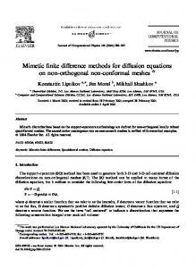
Hildreth (1954) and Hansen and Pledger (1976) only consider the single regressor case, which in the production setting, means there is only one input or that all inputs can be aggregated to a single aggregate input prior to estimating a production function. While this case may seem too restrictive, to be of much use, we include it because: 1) shape restrictions may only be valid for a particular input; 2) it can be solved quickly; and 3) the method to aggregate inputs could be obvious. We can illustrate the first reason by describing wind turbine electricity production where power is the output and wind speed is the only input for which the shape constraints apply. In this case, the production function, which we call the power curve, has a distinct S-shape. Once we estimate the inflection point,13 we can estimate the power curve by a convex function for low wind speeds and a concave function for high wind speeds. Note that other factors influencing power output, e.g., wind direction, wind density, and humidity, do not have a monotonic or convex relationship with power output and thus could enter the model parametrically or via another estimation method. Second, when there is only a single regressor, a complete ordering of observations is possible. This ordering, as shown below, will significantly improve computational performance. Third, in some applications additional restrictions may allow aggregation of multiple inputs to an aggregate input. For example, we can aggregate multiple inputs to a single input when we assume homothetic input sets, Olesen and Ruggiero (2014). Next we consider the estimation of a concave function in two dimensions. Figure 3 shows a CNLS estimate for this example. We randomly generate 50 observations as and

, where

[

]

. Even though there can potentially be one

13

In a power curve or s-shape single-input production function, the inflection point in the input value at which the second derivative changes sign or in other words where the production function changes from being a convex function to a concave function.

11

hyperplane for each observation, CNLS requires only four hyperplanes to minimize the sum of squared errors. Often, CNLS estimation results in significantly fewer hyperplanes than observations, a fact that can be used to improve the computational algorithm (see details in Section 4).

14 12

Output

10 8 6 4 2 0 0

2

4

6

8

10

12

Input Figure 3. CNLS estimation for a 2-dimensional example with 50 randomly generated observations.

GAMS Code This section describes the variables and equation definitions necessary to estimate CNLS in the single input case. The code in Figure 4 should be appended to the bottom of the code from Figure 1. Lines 1-3 define the necessary variables for the CNLS quadratic programming problem. Variable phi corresponds to  defined in (3). GAMS optimizes a single variable and in this case it minimizes sse. In GAMS it is not necessary to include non-negativity constraints, we simply define phi as a positive variable (lines 5-6). Two additional sets are needed to define the monotonicity constraints and concavity constraints in (3), a set that contains i-1 firms and set that contains i-2 firms which are subsets of i and defined as im1(i) and im2(i) in lines 9 and 10 respectively. Three equations are needed to define the CNLS formulation and we name them obj, mono,

and conv1. The equality constraint obj is necessary to define the value of sse. The

equation mono(im1) indicates there are n-1 constraints of type mono defined by indexing over i. 12

Similarly, there are n-2 constraints of the type conv1(imb). Line 28 defines the model which includes all three types of constraints. 1 2 3 4 5 6 7 8 9 10 11 12 13 14 15 16 17 18 19 20 21 22 23 24 25 26 27 28

VARIABLES phi(i) sse

error terms sum of squared errors;

POSITIVE VARIABLES phi ; SETS im1(i) im2(i)

'firms - 1' /1*88/ 'firms - 2' /1*87/ ;

EQUATIONS obj mono(im1) conv1(im2)

objective function regression equation convexity ;

x(i) = data(i,'TOTEX'); * Define Equations obj.. sse =e= sum(i, sqr(y(i)- phi(i)) )

;

mono(im1).. phi(im1) =l= phi(im1+1); conv1(im2).. (phi(im2+1) - phi(im2)) * (x(im2+1) - x(im2)) =l= (phi(im2+2) - phi(im2+1)) * (x(im2+2) - x(im2+1)); MODEL cnls

model / obj, mono, conv1 / ;

Figure 4. GAMS code for CNLS in the single input case.

Matlab Code Matlab uses CVX,14 a modeling system that automatically generates the constraints of CNLS, thus avoiding the need to explicitly enumerate them in matrix form. Figure 5 presents standalone code for CNLS with a single input. Line 1 defines a function that reads in two parameters x and y, which are the n by 1 dimensional input matrix and the n by 1 output vector respectively. The function outputs two values eps (an n by 1 vector of residuals) and phi (an n by 1 vector of functional estimates). Line 2 defines n the number of observations from the parameter y. Line 4 indicates where the code to be read by CVX begins. Line 5 defines the variable for the CNLS problem and its dimensions. Variable phi corresponds to  defined in (3). Line 4 specifies the

14

www.cvxr.com

13

objective function as the 2-norm between the observed value y and the predicted value  . Note that the default value of norm is the 2-norm, so norm(y-phi) and norm(y-phi,2) are equivalent. Line 5 can be omitted, but we include it to make clear where the constraint section begins. The loop in lines 9-11 imposes the (n-1) monotonicity constraints. The loops in lines 13-16 construct (n-2) concavity constraints. Line 19 calculates the residuals called eps.

1 2 3 4 5 6 7 8 9 10 11 12 13 14 15 16 17 18 19

function [eps,phi] = ComputeConcaveSRFn(x,y) n = size(y,1); cvx_begin quiet variable phi(n) minimize(norm(y-phi)) subject to %This loop constructs the monotonicity constraints for i = 1:n-1, phi(i) = ( phi(i+2) - phi(i+1) ) / ( x(i+2) - x(i+1) ); End cvx_end eps = y - phi;

Figure 5. Matlab code for the CNLS in the single input case.

3.2 Convex Nonparametric Least Squares with multiple regressor Kuosmanen (2008) extended Hildreth’s approach to the multivariate setting with a vector-valued x, and named the method convex nonparametric least squares (CNLS). CNLS estimates an unknown production function f belonging to the set of continuous, monotonic increasing and globally concave functions, F2 . We obtain the CNLS estimator of function f as the optimal solution to the infinite dimensional least squares problem n

min  ( yi  f (xi )) 2 f

i 1

subject to f  F2

(4)

14

Note that set F2 includes an infinite number of functions, which makes (4) impossible to solve through brute force trial and error. In general, (4) does not have a unique solution for any arbitrary input vector x, but the estimated values, f(x), for the observed data points

(xi , yi ), i  1,..., n are unique. We solve (4) for the observed data points (xi , yi ), i  1,..., n , by solving the following finite dimensional quadratic programming (QP) problem n

min  ( iCNLS ) 2 α ,β ,ε

i 1

subject to yi   i  βi xi   iCNLS i  i  βi xi   h  βh xi h, i

(5)

βi  0 i where  i and β i define the intercept and slope parameters of the tangent hyperplanes that characterize the underlying true function 15 and symbol  iCNLS denotes the CNLS residual. Kuosmanen (2008) shows the optimal solution to (5) is always equal to the optimal solution of (4) in the sense that the objective function values are equal. The CNLS formulation includes a quadratic objective function and constraints are linear equalities and inequalities; thus it is a quadratic programming problem. However, CNLS is in a particular class of quadratic programming problems which can be solved in polynomial time.16 The first set of equality constraints in (5) appears as a regression type constraint with additional i subscripts on the parameters. These n constraints define the potentially n different hyperplanes which we use to approximate the unknown underlying production function. Typically, n hyperplanes are not needed (see example in section 3.1). Because the production function estimated by the optimal solution to (5) is unique only for the input levels associated with observed data, section 3.3 describes a second step linear program which allows the estimation of a unique lower bound function.

Note in our notation βi xi  i1 xi1  i 2 xi 2  ...  im xim . Further, this formulation is intended to show the relationship to other mathematical models, i.e. classic OLS regression and the Afriat inequalities. For computational purposes, the problem may be reformulated to reduce the number of variables and/or constraints as discussed in Section 4.1. 16 Polynomial time solvable implies efficient solution procedures exist and they scale well with the size of the problem. 15

15

The second set of constraints are the Afriat inequalities, see for example Afriat, (1967, 1972); and Varian (1984). Kuosmanen (2008) notes the Afriat inequalities are the key to modeling concavity in the general multiple regression setting. 17 Figure 6, an enlargement of Figure 3, illustrates the effect of the Afriat inequalities. We note that the Afriat inequalities require that for a specific observation, xi, the estimated functional value using the parameters associated with hyperplane i will be less than or equal to xi evaluated using any other observation’s hyperplane. Thus, all hyperplanes not associated with i must be above i’s hyperplane. In other words, the  and  for all star observations must correspond to the bold hyperplane’s parameters.

Figure 6. A specific hyperplane (shown in black and bold); for all observations (shown in red *) between the thin blue vertical lines, the Afriat inequalities ensure that their estimated hyperplane parameters correspond to the lowest hyperplane on that input interval.

GAMS Code This section describes the variables and equation definitions and constructs the programming model. The code in Figure 7 should be appended to the bottom of the Figure 1 code. Lines 1-4 defines the parameter x and assigns data. Lines 6-10 define the necessary variables for the CNLS For those familiar with DEA, the parameters  i and β i are analogous to u0 and u in the multiplier formulation of DEA. 17

16

quadratic programming problem. alpha and beta correspond to the  and β defined in (5) in the text above, e corresponds to  CNLS in (5), and sse is the objective function value, i.e. the sum of squared errors. Beta is defined as a positive variable (lines 12-13). Three equations are needed to define the CNLS formulation and we name them obj, err, and conv. Equation err(i) indicates there are n constraints of type err defined by indexing over i. Similarly, there are n2 constraints of the type conv(i,h). These are the Afriat constraints we defined above for all pairs of i and h. GAMS optimizes a single variable and in this case it minimizes sse; thus the equality constraint obj is necessary to define the value of sse. Lines 27-28 define the model which includes all three types of constraints, thus we use / all / (in the case that we prefer to include only a subset of constraints, we would use / obj, err, conv /). Line 30 commands GAMS to solve CNLS using quadratically constraint program with the objective of minimizing the variable sse. 1 2 3 4 5 6 7 8 9 10 11 12 13 14 15 16 17 18 19 20 21 22 23 24 25 26 27 28 29 30

PARAMETERS x(i,m) 'inputs of firm i'; * Assign data to variables x(i,m) = data(i,m); VARIABLES alpha(i) beta(i,m) e(i) sse

intercept term input coefficients error terms sum of squared errors;

POSITIVE VARIABLES beta ; EQUATIONS obj objective function err(i) regression equation conv(i,h) convexity ; … * Define Equations obj.. sse =e= sum(i, sqr(e(i)))

;

err(i)..

y(i) =e= alpha(i) + sum(m, beta(i,m)*x(i,m)) + e(i) ;

conv(i,h)..

alpha(i) + sum(m, beta(i,m)*x(i,m)) =l= alpha(h) + sum(m, beta(h,m)*x(i,m));

MODEL CNLS

model / all / ;

SOLVE CNLS using QCP Minimizing sse;

Figure 7. GAMS code for the basic CNLS formulation. 17

Section 4.1 will present an alternative formulation that facilitates the use of disciplined convex programming required by the Matlab-based modeling system CVX.

Illustrative Application: Estimation Results For illustrative purposes we calculate the standard CNLS estimator using GAMS. This section describes the estimates of the production function. For more details regarding the estimates of the inefficiency and noise distributions see Section7.2.1. Table 2 reports some descriptive statistics of the marginal products and elasticities of substitution. The estimated production function is a piece-wise linear function consisting of facets characterized by the variables α and β . Recall we allow α and β to be firm-specific, but in practice, the estimated variables are clustered to a smaller number of facets. Figure 8 illustrates the production possibility set. The hyperplanes are enumerated using the FourierMotzkin method described in Keshvari (2014).

Min 25th percentile Median 75th percentile Max

Marginal Product Labor Capital 0.00 0.00

Elasticity of Substitution Labor/Capital 3.62E-07

0.13 0.13

0.008 0.008

12.18 16.52

0.14 90,644

0.011 75,788

16.62 5,007,995

Table 2. Estimated characteristics of the production function.

We can interpret the values reported in Table 2 as follows. A one euro increase in labor increases the electricity transmitted by 0.13 GWh for the median distributor. Alternatively, a one euro increase in capital has a smaller increase of just 0.008 GWh for the median distributor. Between the 25th percentile and the 75th percentile the effects of labor and capital vary only slightly, indicating there is not much difference in the effectiveness of labor and capital across the majority of firms. Note the min and the max of the marginal product of both labor and capital approach zero and infinite respectively. This characteristic is standard for variable return-to-scale estimators. The elasticity of substitution between labor and capital is 16.52 for the median 18

distributor. This elasticity for the 75th percentile distributor is similar to the median, while the 25th percentile distributor’s elasticity is 12.18. These elasticity values indicate there is not much difference in the rate of substitution of labor for capital across distributors. Again, the min and the max of the elasticity of substitution approaches zero and infinite respectively. This is typical of piece-wise linear approximations, some part of the frontier is only weakly efficient, but this assures the input isoquant remains in the positive orthange.

6,000

Energy (GWh)

5,000 4,000 3,000 2,000 1,000 0 60,000 50,000 40,000 30,000 20,000 10,000

0

CAPEX (1,000 Euros)

0

60,000 50,000 40,000 30,000 20,000 10,000 OPEX (1,000 Euros)

Figure 8. The 3-D production function estimated using CNLS.

3.3 Estimating the Production Function for Unobserved Input Levels CNLS estimates uniquely the output level associated with the observed inputs levels. However, there are multiple optimal solutions to (5) because infinitely many different functions go through





the set of points xi , ˆ(xi ) that minimizes the sum of squared errors. These different solutions imply different frontiers for these regions without observations. To specify unique  (xi ) for x not observed in the data sample, we define a linear program to identify the lower bound of the set of functions that minimize the least squares criteria. Formally, there exists a set of functions

 *  F2 that solve the optimization problem (5). We denote the set of alternate optima n   F2   *  *  arg min  ( yi   (xi )) 2  . f F2 i 1  

19

Kuosmanen (2008) characterizes the lower and upper bounds for the functions  *  F2 . To select among the functions  * , Kuosmanen and Kortelainen (2012) suggest using the minimum extrapolation principle from Banker et al. (1984); thus use the lower bound





k ˆmin (x)  min   βxk   βxk  ˆ(xi ) i  1,..., n

 ,β

(6)

Note that the lower bound function maintains the axioms of monotonicity and concavity.18

GAMS Code This section describes the variables and equation definitions to estimate the lower bound function. The code in Figure 9 should be appended to the bottom of the following collection of code: the code in Figure 1 and followed by the code in Figure 7. Equation (6) reestimates  and β using the observed input data, x i , and the predicted output ˆ(xi ) . Lines 1-4 define the

variables. The variables alphale and betalb are used to represent the reestimates of  and β . The variable objvlb is just an aggregation variable that allows us to minimize the single variable objvlb.

Line 7 imposes monotonicity in the reestimation by restricting β to be nonnegative.

Line 10 defines the variable phihat(i) that will be assigned the value ˆ(xi ) . Because ˆ(xi ) was not previously defined, line 14 calculates the value of ˆ(xi ) . Line 11 defines xk(m), the input vector of the interpolation point of interest, and Lines 15-16 assign values to the vector. Lines 18-20 define the equation names for the linear programming problem that will be used to estimate the lower bound function. Lines 22-25 assign the explicit equations. Note that one linear program needs to be solved for each interpolation point of interest. Lines 27-28 define the model lowerbound which consists of two constraints objle and errle. Line 30 commands GAMS to solve model lowerbound using linear programming methods with the objective of minimizing the variable objvlb.

CNLS The linear program used to calculate the lower bound function fˆmin is equivalent to the DEA estimator under the assumption of variables returns to scale and replacing the observed output levels with the estimated output level fˆ CNLS (xi ) coming from (5).

18

20

1 2 3 4 5 6 7 8 9 10 11 12 13 14 15 16 17 18 19 20 21 22 23 24 25 26 27 28 29 30

VARIABLES alphalb betalb(m) objvlb

intercept term input coefficients objective value;

POSITIVE VARIABLES betale ; PARAMETERS phihat(i) xk(m)

predicted output input level of interest;

* Assign data to variables phihat(i) = alpha.l(i) + sum(m, beta.l(i,m)*x(i,m)); xk('OPEX') = 1000; xk('CAPEX') = 1000; EQUATIONS objle errle(i)

objective value calculation regression equation;

* Assign Equations objle.. objvlb =e= alphalb + sum(m, betalb(m)*xk(m))

;

errle(i).. alphalb + sum(m, betalb(m)*xk(m)) =g= phihat(i); MODEL lowerbound

model / objle, errle / ;

SOLVE lowerbound using LP Minimizing objvlb;

Figure 9. GAMS code for the estimation of the lower envelop.

Matlab Code Figure 10 presents the Matlab code for estimating the lower bound function. Lines 2-4 from Figure 2 and the code from Figure 8 should be inserted into Figure 10 at Line 2. Line 1 defines a function that reads in three parameters x, y, and xk, which are the input matrix and the output vector and input vector of the interpolation point of interest, x k , respectively. The function outputs a vector of residuals eps, vector of functional estimates phi, the slope coefficients from the original CNLS estimation beta1, and the parameters of the reestimated lower bound function hyperplane, alphalb and betalb. Line 3 constructs a vector of length m of zeros which will be used in the monotonicity constraint. Lines 5-6 define the variables. The variables alphalb and betalb

are used to represent the reestimates of  and β . Line 7 specifies the objective function,

is the minimization of   βxk . Line 10 imposes monotonicity in the reestimation by restricting 21

β to be nonnegative. Lines 12-14 define the n equations which assure the estimated hyperplane

is above all the estimated function values, ˆ(xi ) . This linear program needs to be solved once for every interpolated point of interest. 1 2 3 4 5 6 7 8 9 10 11 12 13 14 15

function [eps,phi,beta1,alphalb,betalb] = ComputeConcaveFnLB(x,y,xk) … l2 = zeros(m,1); cvx_begin quiet variable alphalb variable betalb(m,1) minimize(alphalb + betalb(m)*xk(m)) subject to % This line imposes monotonicity by restricting betalb to be non-negative l2 = phi(i); End cvx_end

Figure 10. Matlab code for the estimation of the lower envelop.

4. Computational Improvement Algorithm Direct implementation of (5) in GAMS or in Matlab works well for problems with 50-250 observations, whereas computational improvements, such as those described in this section, are needed for larger problems.19 Although polynomial time algorithms exist, the number of Afriat inequalities in (5)20 grows quadratically in the number of observations. Specifically, adding a new firm to the sample increases the number of unknown parameters by m+2, and the number of Afriat inequality constraints increases by 2n. The effects of adding additional input variables are less severe. Specifically, an additional input variable increases the number of unknown parameters by n, with no impact on the number of constraints. In this section we describe an alternative formulation which is more concise and a computational improvement algorithm proposed by Lee et al. (2013). 21

19

Our experiments with GAMS were performed on a personal computer with an Intel Core i7 CPU 1.60 GHz and 8 GB RAM. The optimization problems were solved in GAMS 23.3 using the CPLEX 12.0 QCP (Quadratically Constrained Program) solver. Our experiments with Matlab were performed on a laptop computer with an Intel Core i5 CPU 2.50 GHz and 4 GB RAM. 20 From this point forward we refer to only equation (5), but issues regarding (5) apply equally to (7) below. 21 Approximation algorithms are also possible strategies, but we focus on calculating the exact solution to the CNLS formulation.

22

4.1 Alternative Formulation Alternative formulations of CNLS are possible. The following formulation facilitates the use of disciplined convex programming required by the Matlab-based modeling system CVX. All other variables and parameters remain as defined previously. Thus

min y    ,β

2

subject to (7)

i  h  βi  xi  xh  i, h i  h βi  0 i

The objective minimizes the L2 norm between y the observed data and  , which is equivalent to minimizing the sum of squared errors. Formulaton (7) can be derived from (5) by eliminate the equality through substitution for  iCNLS in the objective. We replace n decision variables  i with 

using the relationship i i  βi xi . Then we construct the Afriat inequalities by

substituting  for the left-hand side, substituting out  h using  h h  βh xh , and rearranging the terms. This formulation has

inequality constraints,

(one for each observation and dimension of the input vector), and

non-negative constraints decision variables.

Matlab Code Figure 11 shows the code for estimating the concise formulation of CNLS in Matlab. This code should be appended to the bottom of the code presented in Figure 2. Line 1 indicates where the code to be read by CVX begins. Lines 3-4 define the variables for the CNLS problem and their dimensions. Variable phi corresponds to  defined in (7). The variable beta1 is used for β defined in (7). Line 5 specifies the objective function as the 2-norm between the observed value y the observed data and  . Line 8 imposes the monotonicity constraint. In Figure 2, l is

defined as a matrix of size n by m of zeros; thus line 8 imposes that all components of the β matrix must be non-negative. The loops in lines 10-15 construct n(n-1) constraints equivalent to the Afriat inequalities; see (7). The comparison of i and h when i is equal to h is trivially equality, so this formulation avoids generating these constraints.

23

1 2 3 4 5 6 7 8 9 10 11 12 13 14 15 16 17 18

cvx_begin quiet variable phi(n) variable beta1(n,m) minimize(norm(y-phi)) subject to % This line imposes monotonicity by restricting beta1 to be non-negative l = beta1(i,:)*(x(i,:) - x(h,:)).'; end end end cvx_end eps = y - phi;

Figure 11. Matlab code for the basic CNLS formulation.

4.2 Constraint Reduction Technique Lee et al. (2013)’s algorithm uses a constraint reduction technique to identify an initial set of constraints and iteratively add violated constraints until all necessary constraints are included. Specifically, we focus on the sweet spot approach for identifying initial constraints and group addition for adding violated constraints, because this combination allows problems with up to 1,000 firms to be solved. 22 We also note that Hannah and Dunson (2013) have reported promising results implementing an alternative fitting algorithm. Lee et al. constraint reduction technique that iterates between two operations: (A) solving a version of (5) including only a subset of the Afriat inequalities, and (B) verifying whether the obtained solution satisfies all of the Afriat inequalities; if it does then the algorithm terminates, otherwise the initial subset is augmented with some of the violated constraints and the process restarts. We define the following formulation, which Lee et al. refer to as the Relaxed CNLS problem (RCNLS) 22

Lee et al. found that if there were more than 100 observations, the group strategy for adding constraints was always preferred to other methods tested and that the sweet spot strategy’s threshold value could be adjusted based on the number of observations and the dimensionality of the data. In the experiments of Lee et al., they generate input data uniformly and do not correlate the inputs. However, when input variables are correlated CNLS becomes easier to solve. Thus, in observed data where the inputs are typically highly correlated, the computational improvement will allow problems even larger than 1,000 observations to be solved.

24

∑ Subject to for

for

where

is a subset of all the observation pairs and thus the concavity constraints (8b) are a

subset of all the Afriat inequalities defined in (5). Specifically, 1. Let

and let

be a subset of the observation pairs.

2. Solve RCNLS to find an initial solution, 3. Do until

satisfies all concavity constraints (equations (8b)):

3.1 Select a subset of the concavity constraints that and let

violates

be the corresponding observation pairs.

3.2 Set 3.3 Solve RCNLS to obtain solution 3.4 Set This algorithm requires methods to specify

(the initial constraints) and

(the violated

constraints). The next section gives the details.

Selecting Initial Constraints – the Sweet Spot Method We begin by recognizing that the number of unique hyperplanes to construct a CNLS production function is generally much lower than

as shown in section 3.1. In the optimal solution of

CNLS (5), the concavity constraints that are satisfied at equality correspond to pairs of observations that share a hyperplane in the CNLS function. Because any particular hyperplane is only used to construct part of the lower bound function in a particular region, it is perhaps obvious that observations that share the same hyperplane should be close together under some distance metric. To validate this intuition, we follow Lee et al. (2013) and generate 300

25

observations of a two-input single-output equation, observations,

. We randomly sample

, from a uniform [1,10] distribution and draw

from a normal distribution

with a standard deviation of 0.7. Then we solve both the CNLS problem (5) and the additional linear program problem (6) to identify the constraints that hold with equality in (6), the necessary constraints. The two histograms in Figure 12 show the Euclidean distances between a selected observation’s input vector and all other observations’ input vectors (in black) and the distances between a selected observation’s input vector and all other observations’ input vectors corresponding to the necessary concavity constraints (in white). 50 45

Pairs of Observations

40 35 30 25 20 15 10 5 0 0

1

2

3

4

5

6

7

8

9

10

11

12

Distance Histogram of the distances between all pairs related to one particular observation that correspond to relevant concavity constraints Histogram of the distances between all pairs related to one particular observation

Figure 12. The concavity constraints corresponding to nearby observations are significantly more likely to be necessary23 than those corresponding to distant observations. (Reproduced with permission from Figure 2 in Lee et al. (2013)).

The results of the simulation motivates the development of the sweet spot approach defined as calculating the Euclidean distance between all pairs of observations, i and h, and including the concavity constraints corresponding to the observations whose distance is less than a prespecified threshold value

(distance percentile parameter). Thus, the “sweet spot” is the range

between the zeroth percentile and the 23

percentile. Empirically, Lee et al. find that an effective

The term necessary concavity constraints and relevant concavity constraints can be used interchangeable.

26

value for

is the 3rd percentile of the distances. However, adjusting

based on the number of

observations and the dimensionality of the problem improves the algorithm’s performance, i.e. as the number of inputs increases,

should decrease. Lee et al. also note that the relationship

between the most effective value of

and the number of observations is not monotonic. In their

Monte Carlo simulations, Lee et al. find that setting

to zero is effective when the number of

observations is 200 to 400 and the number of inputs is 5 to 8.24 They conclude that a higher dimensionality (number of inputs) is needed to justify setting

to zero as the number of

observations deviates further from 300.

Selecting Violated Constraints While Lee et al. (2013) suggest three strategies for adding violated constraints, we focus on the most effective strategy: adding a group of violated constraints, CNLS+G. This strategy selects for each observation , the most violated constraint among the n-1 concavity constraints related to observation . We note that it can add as many as n constraints in each iteration.



max it  it xi -  ht  ht xi h

  0

i  1,..., n

(9)

Adding a group of violated constraints balances the number of iterations of the algorithm against the size of the RCNLS problem solved in each iteration.

GAMS Code The use of GAMS to implement the CNLS+G method is complicated, since the code requires addition formulations of the CNLS quadratic optimization program (see appendix A for the full code). Figure 13 describes the implementation of the sweet spot method. Lines 2-5 define the equation names. Lines 8-13 define the specific equation structure of the quadratic programming problem that is solved as the initial solution to RCNLS. Line 15 defines the model CNLS1 which is the initial solution of RCNLS; the subset of the Afriat constraints included in the sweet spot also is included in solving RCNLS. Line 17 flags the constraints that are close in terms of distance. We calculate the data distance and distcut offline and read them into GAMS. Line 19 triggers GAMS to solve model CNLS1 using quadratic constrained programming (qcp)

24

Setting to zero implies that the set V is empty and (8) is solved with only the (8a) and (8c) constraints. V still grows via the addition of violated constraints in the algorithm.

27

methods; typically, we use either CPLEX or MINOS.25 For the iterative strategy of adding a group of violated constraints, the GAMS code in Appendix A shows an implementation. 1 2 3 4 5 6 7 8 9 10 11 12 13 14 15

* equations for initial CNLS+G (objective function and constraints) EQUATIONS QSSE1 objective=sum of squares of errors QREGR1(k) regression equation ConcavB1(k,h) concavity constraints for sweet spot; *initial CNLS+G model QSSE1.. SS1 =e= sum(k,E1(k)*E1(k)); QREGR1(k).. dataA(k,"Y") =e= A1(k)+sum(inp,B1(k,inp)*dataA(k,inp))+ E1(k); ConcavB1(k,h)$(Cutactive(k,h)).. A1(k)+sum(inp,B1(k,inp)*dataA(k,inp)) =l= A1(h)+sum(inp,B1(h,inp)*dataA(k,inp)); Model CNLS1 /QSSE1, QREGR1, ConcavA1, ConcavB1 / …

16 17

*find concavity constraint in sweet spot Cutactive(k,h)=yes$(distance(k,h)