particularly generic and powerful method, known as the Support Vector Machine (SVM) has ..... marketing applications, can work in multiple dimensions, and is ...
Support Vector Machines for Business Applications Brian C. Lovell† and Christian J Walder†‡ †
The University of Queensland and ‡ Max Planck Institute, Tübingen {lovell, walder}@itee.uq.edu.au
Introduction Recent years have seen an explosive growth in computing power and data storage within business organisations. From a business perspective, this means that most companies now have massive archives of customer and product data and more often than not these archives are far too large for human analysis. An obvious question has therefore arisen, “How can one turn these immense corporate data archives to commercial advantage?” To this end, a number of common applications have arisen, from predicting which products a customer is most likely to purchase, to designing the perfect product based on responses to questionnaires. The theory and development of these processes has grown into a discipline of its own, known as Data Mining, which draws heavily on the related fields of Machine Learning, Pattern Recognition, and Mathematical Statistics. The Data Mining discipline is still developing however, and a great deal of suboptimal and ad hoc analysis is being done. This is partly due to the complexity of the problems, but is also due to the vast number of available techniques. Even the most fundamental task in Data Mining – that of inductive inference, or making predictions based on examples, can be tackled by a great many different techniques. Some of these techniques are very difficult to tailor to a specific problem and require highly skilled human design; others are more generic in application and can be treated more like the proverbial “black box”. One particularly generic and powerful method, known as the Support Vector Machine (SVM) has proven to be both easy to apply and capable of producing results that range from good to excellent in comparison to other methods. While application of the method is relatively straightforward, the practitioner can still benefit greatly from a basic understanding of the underlying machinery. Unfortunately most available tutorials on SVMs do require a very solid mathematical background, so we have written this chapter to make SVMs accessible to a wider community. This chapter comprises a basic background on the problem of induction, followed by the main sections. In the first section we introduce the concepts and equations on which the SVM is based in an intuitive manner and to identify the relationship between the SVM and some of the other popular analysis methods. In the second section we survey some interesting applications of SVMs on practical real world problems. Finally, the third section provides a set of guidelines and rules of thumb for applying the tool, with a pedagogical example that is designed to demonstrate everything that the SVM newcomer requires in order to immediately apply the tool to a specific problem domain. The chapter is intended as a brief introduction to the field that introduces the ideas, methodologies, as well as a hand-on introduction to freely available software, allowing the reader to rapidly determine the effectiveness of SVMs for their specific domain.
Background SVMs are most commonly applied to the problem of inductive inference, or making predictions based on previously seen examples. To illustrate what is meant by this, let us consider the data presented in Tables 1 and 2. We see here an example of the problem of inductive inference, more specifically that of supervised learning. In supervised learning we are given a set of input data along with their corresponding labels. The input data comprises a number of examples about which several attributes are known (in this case, age, income etc). The label indicates which class a particular example belongs to. In the example above, the label tells us whether or not a given person has broadband internet connection to their home. This is called a binary classification problem because there are only two possible classes. In the second table, we are given the attributes for a different set of consumers, for whom the true class labels are unknown. Our goal
is to infer from the first table the most likely labels for the people in the second table, that is, whether or not they have a broadband internet connection to their home. Age
Income
30 50 16 35
$56,000 / yr $60,000 / yr $2,000 / yr $30,000 / yr
Years of Education 16 12 11 12
Gender male female male male
Broadband Home Internet Connection? Yes Yes No No
Table 1: training or labelled set The dataset in Table 1 contains demographic information for four randomly selected people. These people were surveyed to determine whether or not they had a broadband home internet connection. Age
Income
40 29
$48,000 / yr $60,000 / yr
Years of Education 17 18
Gender male female
Broadband Home Internet Connection? unknown unknown
Table 2: unlabelled set The dataset in Table 2 contains demographic information for people who may or may not be good candidates for broadband internet connection advertising. The question arising is, “Which of these people is likely to have broadband internet connection at home?” In the field of data mining, we often refer to these sets by the terms test set, training set, validation set, and so on, but there is some confusion in the literature about the exact definitions of these terms. For this reason we avoid this nomenclature, with the exception of the term training set. For our purposes, the training set shall be all that is given to us in order to infer some general correspondence between the input data and labels. We will refer to the set of data for which we would like to predict the labels as the unlabelled set. A schematic diagram for the above process is provided in Figure 1. In the case of the SVM classifier (and most other learning algorithms for that matter), there are a number of parameters which must be chosen by the user. These parameters control various aspects of the algorithm, and in order to yield the best possible performance, it is necessary to make the right choices. The process of choosing parameters that yield good performance is often referred to as model selection. In order to understand this process, we have to consider what it is that we are aiming for in terms of classifier performance. From the point of view of the practitioner, the hope is that the algorithm will be able to make true predictions about unseen cases. Here the true values we are trying to predict are the class labels of the unlabelled data. From this perspective it is natural to measure the performance of a classifier by the probability of its misclassifying an unseen example. It is here that things become somewhat less straightforward, however, due to the following dilemma. In order to estimate the probability of a misclassification, we need to know the true underlying probability distributions of the data that we are dealing with. If we actually knew this, however, we wouldn’t have needed to perform inductive inference in the first place! Indeed knowledge of the true probability distributions allows us to calculate the theoretically best possible decision rule corresponding to the socalled Bayesian classifier (Duda et al 2001). In recent years, a great deal of research effort has gone into developing sophisticated theories that make statements about the probability of a particular classifier making errors on new unlabelled cases — these statements are typically referred to as generalization bounds. It turns out however, that the research has a long way to go, and in practice one is usually forced to determine the parameters of the learning algorithm by much more pragmatic means. Perhaps the most straightforward of these methods involves estimating the probability of misclassification using a set of real data for which the class labels are known — to do this one simply compares the labels predicted by the learning algorithm to the true known labels. The estimate of
misclassification probability is then given by the number of examples for which the algorithm made an error (that is, predicted a label other than the true known label) divided by the number of examples which were tested in this manner.
Labelled Training Data
Unlabelled Data Predicted Labels
Learning Algorithm (SVM)
Decision Rule
Figure 1: The inductive inference process in schematic form. Based on a particular training set of examples with labels, the learning algorithm constructs a decision rule which can then be used to predict the labels of new unlabelled examples. Some care needs to be taken however, in how this procedure is conducted. A common pitfall for the inexperienced analyst involves making this estimate of misclassification probability using the training set from which the decision rule itself was inferred. The problem with this approach is easily seen from the following simple decision rule example. Imagine a decision rule that makes label predictions by way of the following procedure (sometimes referred to as the notebook classifier): The notebook classifier decision rule: We wish to predict the label of the example X. If X is present in the training set, make the prediction that its label is the same as the corresponding label in the training set. Otherwise, toss a coin to determine the label. For this method, while the estimated probability of misclassification on the training set will be zero, it is clear that for most real world problems the algorithm will perform no better than tossing a coin! The notebook classifier is a commonly used example to illustrate the phenomenon of overfitting — which refers to situations where the decision rule fits the training set well, but does not generalize well to previously unseen cases. What we are really aiming for is a decision rule that generalizes as well as possible, even if this means that it cannot perform as well on the training set. Cross-validation: So it seems that we need a more sophisticated means of estimating the generalization performance of our inferred decision rules, if we are to successfully guide the model selection process. Fortunately there is a more effective means of estimating the generalization performance based on the training set. This procedure, which is referred to as cross-validation or more specifically n-fold cross validation, proceeds in the following manner (Duda et al 2001): 1. 2. 3. 4. 5.
Split the training set into n equally sized and disjoint subsets (partitions), numbered 1 to n. Construct a decision function using a conglomerate of all the data from subsets 2 to n. Use this decision function to predict the labels of the examples in subset number 1. Compare the predicted labels to the known labels in subset number 1. Repeat steps 1 through 4 a further (n-1) times, each time testing on a different subset, and always excluding that subset from training.
Having done this, we can once again divide the number of misclassifications by the total number of training examples to get an estimate of the true generalization performance. The point is that since we have avoided checking the performance of the classifier on examples that the algorithm had already “seen”, we have calculated a far more meaningful measure of classifier quality. Commonly used values for n are 3 and 10 leading to so called 3-fold and 10-fold cross-validation. Now, while it is nice to have some idea of how well our decision function will generalize, we really want to use this measure to guide the model selection process. If there are only, say, two parameters to choose for the classification algorithm, it is common to simply evaluate the generalization performance (using cross validation) for all combinations of the two parameters, over some reasonable range. As the number of parameters increases, however, this soon becomes infeasible due to the excessive number of parameter combinations. Fortunately one can often get away with just two parameters for the SVM algorithm, making this relatively straight-forward model selection methodology widely applicable and quite effective on real world problems. Now that we have a basic understanding of what supervised learning algorithms can do, as well as roughly how they should be used and evaluated, it is time to take a peek under the hood of one in particular, the SVM. While the main underlying idea of the SVM is quite intuitive, it will be necessary to delve into some mathematical details in order to better appreciate why the method has been so successful.
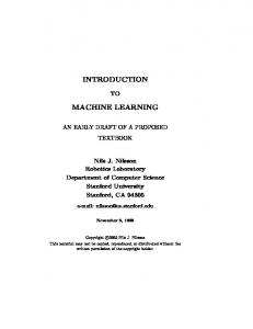
Main Thrust of the Chapter The SVM is a supervised learning algorithm that infers from a set of labeled examples a function that takes new examples as input, and produces predicted labels as output. As such the output of the algorithm is a mathematical function that is defined on the space from which our examples are taken, and takes on one of two values at all points in the space, corresponding to the two class labels that are considered in binary classification. One of the theoretically appealing things about the SVM is that the key underlying idea is in fact extremely simple. Indeed, the standard derivation of the SVM algorithm begins with possibly the simplest class of decision functions: linear ones. To illustrate what is meant by this, Figure 2 consists of three linear decision functions that happen to be correctly classifying some simple 2D training sets.
Figure 2: A simple 2D classification task, to separate the black dots from the circles. Three feasible but different linear decision functions are depicted, whereby the classifier predicts that any new samples in the gray region are black dots, and those in the white region are circles. Which is the best decision function and why? Linear decision functions consist of a decision boundary that is a hyperplane (a line in 2D, plane in 3D, etc) separating the two different regions of the space. Such a decision function can be expressed by a mathematical function of an input vector x, the value of which is the predicted label for x (either +1 or -1). The linear classifier can therefore be written as
g (x) = sign( f (x)) where f (x) =< w, x > +b.
In this way we have parameterized the function by the weight vector w and the scalar b. The notation denotes the inner or scalar product of w and x, defined by d
< w, x >= ∑ wi xi i =1
where d is the dimensionality, and wi is the i-th component of w, where w is of the form (w1, w2, … wd). Having formalized our decision function, we can now formalize the problem which the linear SVM addresses: Given a training set of vectors x1, x2, … xn with corresponding class membership labels y1, y2, … yn that take on the values +1 or -1, choose parameters w and b of the linear decision function that generalizes well to unseen examples. Perceptron Algorithm: Probably the first algorithm to tackle this problem was the Perceptron algorithm (Rosenblatt 1958). The Perceptron algorithm simply used an iterative procedure to incrementally adjust w and b until the decision boundary was able to separate the two classes of the training data. As such, the Perceptron algorithm would give no preference between the three feasible solutions in Figure 2 — any one of the three could result. This seems rather unsatisfactory as most people would agree that the rightmost decision function is the superior one. Moreover, this intuitive preference can be justified in various ways, for example by considering the effect of measurement noise on the data — small perturbations of the data could easily change the predicted labels of the training set in the first two examples, whereas the third is far more robust in this respect. In order to make use of this intuition, it is necessary to state more precisely why we prefer the third classifier: We prefer decision boundaries that not only correctly separate two classes in the training set, but lie as far from the training examples as possible. This simple intuition is all that is required to lead to the linear SVM classifier, which chooses the hyperplane that separates the two classes with the maximum margin. The margin is just the distance from the hyperplane to the nearest training example. Before we continue, it is important to note that while the above example shows a 2D dataset, which can be conveniently represented by points in a plane, in fact we will typically be dealing with higher dimensional data. For example, the example data in Table 1 could easily be represented as points in four dimensions as follows.
x1 = [ x2 = [ x3 = [ x4 = [
30 50 16 35
56000 60000 2000 30000
16 12 11 12
0 1 0 0
1] ; 0] ; 1] ; 1] ;
y1 = +1 y2 = +1 y3 = -1 y4 = -1
Actually, there are some design decisions to be made by the practitioner when translating attributes into the above type of numerical format, which we shall touch on in the next section. For example here we have mapped the male/female column into two new numerical indicators. For now, just note that we have also listed the labels y1 to y4 which take on the value +1 or -1, in order to indicate the class membership of the examples (that is, yi = 1 means that xi has broadband home internet connection). In order to easily find the maximum margin hyperplane for a given data set using a computer, we would like to write the task as an optimization problem. Optimization problems consist of an objective function, which we typically want to find the maximum or minimum value of, along with a set of constraints, which are conditions that we must satisfy while finding the best value of the objective function. A simple example is to minimize x2 subject to the constraint that 1 ≤ x ≤ 2. The solution to this example optimization problem happens to be x = 1. To see how to compactly formulate the maximum margin hyperplane problem as an optimization problem, take a look at Figure 3.
+b= –1
+b=+1 +b=0
Figure 3: Linearly separable classification problem The Figure shows some 2D data drawn as circles and black dots, having labels +1 and –1 respectively. As before, we have parameterized our decision function by the vector w and the scalar b, which means that, in order for our hyperplane to correctly separate the two classes, we need to satisfy the following constraints:
< w, x i > +b > 0, for all yi = 1 < w, x i > +b < 0, for all yi = −1 To aid understanding, the first constraint above may be expressed as: “ + b must be greater than zero, whenever yi is equal to one.” It is easy to check that the two sets of constraints above can be combined into the following single set of constraints:
(< w, x i > +b) yi > 0, i = 1...n However meeting this constraint is not enough to separate the two classes optimally – we need to do so with the maximum margin. An easy way to see how to do this is the following. First note that we have plotted the decision surface as a solid line in Figure 3, which is the set satisfying:
< w, x > +b = 0.
(1)
The set of constraints that we have so far is equivalent to saying that these data must lie on the correct side (according to class label) of this decision surface. Next notice that we have also plotted as dotted lines two other hyperplanes, which are the hyperplanes where the function + b is equal to -1 (on the lower left) and +1 (on the upper right). Now, in order to find the maximum margin hyperplane, we can see intuitively that we should keep the dotted lines parallel and equidistant to the decision surface, and maximize their distance from one another, while satisfying the constraint that the data lie on the correct side of the dotted lines associated with that class. In mathematical form, the final clause of this sentence (the constraints) can be written as
yi (< w, x i > +b) > 1, i = 1...n. All we need to do then is to maximize the distance between the dotted lines subject to the constraint set above. To aid in understanding, one commonly used analogy is to think of these data points as nails partially driven into a board. Now we successively place thicker and thicker pieces of timber between the nails representing the two classes until the timber just fits —the centreline of the timber now represents the
optimal decision boundary.
It turns out that this distance is equal to
maximizing 2 / < w, w > is the same as minimizing < w, w
2 / < w, w > , and since
> , we end up with the following
optimization problem, the solution of which yields the parameters of the maximum margin hyperplane. The term ½ in the objective function below can be ignored as it simply makes things neater from a certain mathematical point of view: 1 min w ⋅ w w ,b 2 such that yi (w ⋅ x i + b) ≥ 1 for all i = 1, 2,..., m
The above problem is quite simple, but it encompasses the key philosophy behind the SVM — maximum margin data separation. If the above problem had been scribbled onto a cocktail napkin and handed to the pioneers of the Perceptron back in the 1960’s, then the Machine Learning discipline would probably have progressed a great deal further than it has to date! We cannot relax just yet however, as there is a major problem with the above method: What if these data are not linearly separable? That is if it is not possible to find a hyperplane that separates all of the examples in each class from all of the examples in the other class? In this case there would be no combination of w and b that could ever satisfy the set of constraints above, let alone do so with maximum margin. This situation is depicted in Figure 4, where it becomes apparent that we need to soften the constraint that these data lie on the correct side of the +1 and -1 hyperplanes, that is we need to allow some, but not too many data points to violate these constraints by a preferably small amount. This alternative approach turns out to be very useful not only for datasets that are not linearly separable, but also, and perhaps more importantly, in allowing improvements in generalization.
+b= –1
+b=+1 +b=0
Figure 4: Linearly inseparable classification problem Usually when we start talking about vague concepts such as “not too many” and “a small amount”, we need to introduce a parameter into our problem, which we can vary in order to balance between various goals and objectives. The following optimization problem, known as the 1-norm soft margin SVM, is probably the one most commonly used to balance the goals of maximum margin separation, and correctness of the training set classification. It achieves various trade-offs between these goals for various values of the parameter C, which is usually chosen by cross-validation on a training set as discussed earlier.
m 1 min w ⋅ w + C ∑ ξi w ,b , ξ 2 i =1 such that yi (w ⋅ x i + b) + ξi ≥ 1
(2)
for all i = 1, 2,..., m.
The easiest way to understand this problem is by comparison with the previous formulation that we gave, which is known as the hard margin SVM, in reference to the fact that the margin constraints are “hard”, and are not allowed to be violated at all. First note that we have an extra term in our objective function that is equal to the sum of the ξi’s. Since we are minimizing the objective function, it is safe to say that we are looking for a solution that keeps the ξi values small. Moreover, since the ξ term is added to the original objective function after multiplication by C, we can say that as C increases we care less about the size of the margin, and more about keeping the ξi’s small. The true meaning of the ξi’s can only be seen from the constraint set, however. Here, instead of constraining the function yi( + b) to be greater than 1, we constrain it to be greater than 1 - ξi. That is, we allow the point xi to violate the margin by an amount ξi. Thus, the value of C trades between how large of a margin we would prefer, as opposed to how many of the training set examples violate this margin (and by how much). So far, we have seen that the maximally separating hyperplane is a good starting point for linear classifiers. We have also seen how to write down the problem of finding this hyperplane as an optimization problem consisting of an objective function and constraints. After this we saw a way of dealing with data that is not linearly separable, by allowing some training points to violate the margin somewhat. The next limitation we will address is in the form of solutions available. So far we have only considered very simple linear classifiers, and as such we can only expect to succeed in very simple cases. Fortunately it is possible to extend the previous analysis in an intuitive manner, to more complex classes of decision functions. The basic idea is illustrated in Figure 5.
Figure 5: An example of a mapping Ф to a feature space in which the data become linearly separable. The example in Figure 5 shows on the left a data set that is not linearly separable. In fact, the data is not even close to linearly separable, and one could never do very well with a linear classifier for the training set given. In spite of this, it is easy for a person to look at the data and suggest a simple elliptical decision surface that ought to generalize well. Imagine however that there is a mapping Ф which transforms these data to some new, possibly higher dimensional space, in which the data is linearly separable. If we knew Ф then we could map all of the data to the feature space, and perform normal SVM classification in this space. If we can achieve a reasonable margin in the feature space, then we can expect a reasonably good generalization performance, in spite of a possible increase in dimensionality.
The last sentence of the previous paragraph is far deeper than it may first appear. For some time, Machine Learning researchers have feared the curse of dimensionality, a name given to the widely-held belief that if the dimension of the feature space is large in comparison to the number of training examples, then it is difficult to find a classifier that generalizes well. It took the theory of Vapnik and Chervonenkis (Vapnik 1998) to put a serious dent in this belief. In a nutshell, they formalized and proved the last sentence of the previous paragraph, and thereby paved the way for methods that map data to very high dimensional feature spaces where they then perform maximum margin linear separation. Actually, a tricky practical issue also had to be overcome before the approach could flourish: if we map to a feature space that is too high in dimension, then it will become impossible to perform the required calculations (that is, to find w and b) — that is, it would take too long on a computer. It is not obvious how to overcome this difficulty, and it took until 1995 for researchers to notice the following elegant and quite remarkable possibility. The usual way of proceeding is to take the original soft margin SVM, and convert it to an equivalent Lagrangian dual problem. The derivation is not especially enlightening however, so we will skip to the result, which is that the solution to the following dual or equivalent problem gives us the solution to the original SVM problem. The dual problem, which is to be solved by varying the αι’s, is as follows (Vapnik 1998) min α
m 1 m yi y jα iα j (xi ⋅ x j ) −∑ α i ∑ 2 i , j =1 i =1
such that
m
∑ yα i
i =1
i
=0
(3)
0 ≤ α i ≤ C, i = 1, 2,..., m.
The αι’s are known as the dual variables, and they define the corresponding primal variables w and b by the following relationships: m
w = ∑ α i yi x i i =1
α i ( yi (< w, x i > +b) − 1) = 0 Note that by the linearity of the inner product (that is, the fact that = + ), we can write the decision function in the following form: m
f (x) =< w, x > +b = ∑ α i yi < x i , x > +b i =1
Recall that it is the sign of f(x) that gives us the predicted label of x. A quite remarkable thing is that in order to determine the optimal values of the αι’s and b, and also to calculate f(x), we do not actually need to know any of the training or testing vectors, we only need to know the scalar value of their inner product with one another. This can be seen by noting that the vectors only ever appear by way of their inner product with one another. The elegant thing is that rather than explicitly mapping all of the data to the new space and performing linear SVM classification, we can operate in the original space, provided we can find a socalled kernel function k(.,.) which is equal to the inner product of the mapped data. That is, we need a kernel function k(.,.) satisfying:
k (x, y ) =< Φ (x), Φ (y ) > In practice, the practitioner need not concern him or herself with the exact nature of the mapping Ф. In fact, it is usually more intuitive to concentrate on properties of the kernel functions anyway, and the prevailing wisdom states that the function k(x,y) should be a good measure of the similarity of the vectors x and y. Moreover, not just any function k can be used — it must also satisfy certain technical conditions, known as
Mercer’s conditions. This procedure of implicitly mapping the data via the function k is typically often called the kernel trick and has found wide application after being popularized by the success of the SVM (Schölkopf, & Smola 1998). The two most widely used kernel functions are the following. Polynomial Kernel
k(x, y) = (< x, y > + 1) d
The polynomial kernel is valid for all positive integers d ≥ 1. The kernel corresponds to a mapping Ф that computes all degree d monomial terms of the individual vector components of the original space. The polynomial kernel has been used to great effect on digit recognition problems. Gaussian Kernel
k(x, y) = exp( -
|| x − y ||2
σ2
)
The Gaussian kernel, which is similar to the Gaussian probability distribution from which it gets its name, is one of a group of kernel functions known as radial basis functions (RBFs). RBFs are kernel functions that depend only on the geometric distance between x and y. The kernel is valid for all non-zero values of the kernel width σ, and corresponds to a mapping Ф into an infinite dimensional, and therefore somewhat less interpretable, feature space. Nonetheless, the Gaussian is probably the most useful and commonly used kernel function. Now that we know the form of the SVM dual problem, as well as how to generalize it using kernel functions, the only thing left is to see is how to actually solve the optimization problem, in order to find the αι’s. The optimization problem is one example of a class of problems known as Quadratic Programs (QPs). The term program, as it is used here, is somewhat antiquated and in fact means a “mathematical optimization problem”, not a computer program. Fortunately there are many computer programs that can solve QP’s such as this, these computer programs being known as Quadratic Program (QP) solvers. An important factor to note here is that there is considerable structure in the QP that arises in SVM training, and while it would be possible to use almost any QP solver on the problem, there are a number of sophisticated software packages tailored to take advantage of this structure, in order to decrease the requirements of computer time and memory. One property of the SVM QP that can be taken advantage of is its sparsity — the fact that in many cases, at the optimal solution most of the αι’s will equal zero. It is interesting to see what this means in terms of the decision function f(x): those vectors with αι = 0 do not actually enter into the final form of the solution. In fact, it can be shown that one can remove all of the corresponding training vectors before training even commences, and get the same final result. The vectors with non-zero values of αι are known as the Support Vectors, a term that has its root in the theory of convex sets. As it turns out, the Support Vectors are the “hard” cases – the training examples that are most difficult to classify correctly (and that lie closest to the decision boundary). In our previous practical analogy, the support vectors are literally the nails that support the block of wood! Now that we have an understanding of the machinery underlying it, we will soon proceed to solve a practical problem using the freely available SVM software package libSVM written by Hsu and Lin.
Relationship to Other Methods We noted in the introduction that the SVM is an especially easy to use method that typically produces good results even when treated as a processing “black box”. This is indeed the case, and to better understand this it is necessary to consider what is involved in using some other methods. We will focus in detail on the extremely prevalent class of algorithms known as artificial neural networks, but first we provide a brief overview of some other related methods. Linear Discriminant Analysis (Hand 1981, Weiss & Kulikowski 1991) is widely used in business and marketing applications, can work in multiple dimensions, and is well-grounded in the mathematical literature. It nonetheless has two major drawbacks. The first is that linear discriminant functions, as the
name implies, can only successfully classify linearly separable data thus limiting their application to relatively simple problems. If we extend the method to higher order functions such as quadratic discriminators, generalization suffers. Indeed such degradation in performance with increased numbers of parameters corroborated the belief in the “curse of dimensionality” finally disproved by Vapnik (Vapnik, 1998). The second problem is simply that generalization performance on real problems is usually significantly worse than either decision trees or artificial neural networks (e.g., see the comparisons in Weiss & Kulikowski 1991). Decision Trees are commonly used in classification problems with categorical data (Quinlan 1993), although it is possible to derive categorical data from ordinal data by introducing binary valued features such as “age is less than 20”. Decision trees construct a tree of questions to be asked of a given example in order to determine the class membership by way of class labels associated with leaf nodes of the decision tree. This approach is simple and has the advantage that it produces decision rules that can be interpreted by a human as well as a machine; however the SVM is more appropriate for complex problems with a many ordinal features. Nearest Neighbour methods are very simple and therefore suitable for extremely large data sets. These methods simply search the training data set for the k examples that are closest (by the criteria of Euclidean distance for example) to the given input. The most common class label that associated with these k is then assigned to the given query example. When the training and testing computation times are not so important however, the discriminative nature of the SVM will usually yield significantly improved results. Artificial Neural Network (ANN) algorithms have become extremely widespread in the area of data mining and pattern recognition (Bishop, 1995). These methods were originally inspired by the neural connections that comprise the human brain – the basic idea being that in the human brain many simple units (neurons) are connected together in a manner that produces complex, powerful behaviour. To simulate this phenomenon, neurons are modeled by units whose output y is related to the input x by some activation function g by the relationship y = g(x). These units are then connected together in various architectures, whereby the output of a given unit is multiplied by some constant weight and then fed forward as input to the next unit, possibly in summation with a similarly scaled output from some other unit(s). Ultimately all of the inputs are fed to one single final unit, the output of which is typically compared to some threshold in order to produce a class membership prediction. This is a very general framework that provides many avenues for customisation: • • • •
Choice of activation function Choice of network architecture (number of units and the manner in which they are connected) Choice of the “weights” by which the output of a given unit is multiplied to produce the input of another unit. Algorithm for determining the weights given the training data.
In comparison to the SVM, both the strength and weakness of the ANN lies in it’s flexibility – typically a considerable amount of experimentation is required in order to achieve good results, and moreover since the optimization problems that are typically used to find the weights of the chosen network are non-convex, many numerical tricks are required in order to find a good solution to the problem. Nonetheless, given sufficient skill and effort in engineering a solution with an ANN, one can often tailor the algorithm very specifically to a given problem in a process that is likely to eventually yield superior results to the SVM. Having said this, there are cases, for example in handwritten digit recognition, in which SVM performance is on par with highly engineered ANN solutions (DeCoste 2002). By way of comparison, the SVM approach is likely to yield a very good solution with far less effort than is required for a good ANN solution.
Practical Application of the SVM As we have seen, the theoretical underpinnings of the SVM are very compelling, especially since the algorithm involves very little trial and error, and is easy to apply. Nonetheless, the usefulness of the
algorithm can only be borne out by practical experience, and so in this sub-section we survey a number of studies that use the SVM algorithm in practical problems. Before we mention such specific cases, we first identify the general characteristics of those problems to which the SVM is particularly well suited. One key consideration is that in its basic form the SVM has limited capacity to deal with large training data sets. Typically the SVM can only handle problems of up to approximately 100,000 training examples before approximations must be made in order to yield reasonable training times. Having said this, the training times depend only marginally on the dimensionality of the features – it is often said that SVMs can often defy the so-called curse of dimensionality –the difficulty that often occurs when the dimensionality is high in comparison with the number of training samples. It should also be noted that, with the exception of the string kernel case, the SVM is most naturally suited to ordinal features rather than categorical ones, although as we shall see in the next Section, it is possible to handle both cases. Before turning to some specific business and marketing cases, it is important to note that some of the most successful applications of the SVM have been in image processing – in particular handwritten digit recognition (DeCoste 2002) and face recognition (Osuna 1997). In these areas, a common theme of the application of SVMs is not so much increased accuracy, but rather a greatly simplified design and implementation process. As such, when considering popular areas such as face recognition, it is important to understand that very simple SVM implementations are often competitive with the complex and highly tuned systems that were developed over a longer period prior to the advent of the SVM. Another interesting application area for SVMs is on string data, for example in text mining or the analysis of genome sequences (Joachims 2002). The key reason for the great success of SVMs in this area is the existence of “string kernels” – these are kernel functions defined on strings that elegantly avoid many of the combinatoric problems associated with other methods, whilst having the advantage over generative probability models such as the Hidden Markov Model that the SVM learns to discriminate between the two classes via the maximisation of the margin. The practical use of text categorisation systems is extremely widespread, with most large enterprises relying on such analysis of their customer interactions in order to provide automated response systems that are nonetheless tailored to the individual. Furthermore, the SVM has been successfully used in a study of text and data mining for direct marketing applications (Cheung 2003) in which relatively limited customer information was automatically supplanted with the preferences of a larger population, in order to determine effective marketing strategies. To conclude this survey note that while the majority of the marketing teams do not publish their methodologies, since many of the important data mining software packages (for example Oracle Data Mining and SAS Enterprise Miner) have incorporated the SVM, it is likely that there is a significant and increasing use of the SVM in industrial settings.
A Worked Example In “A Practical Guide to Support Vector Classification” (Chang et al 2003) a simple procedure for applying the SVM classifier is provided for inexperienced practitioners of the SVM classifier. The procedure is intended to be easy to follow, quick, and capable of producing reasonable generalization performance. The steps they advocate can be paraphrased as follows: 1. 2. 3. 4. 5.
Convert the data to the input format of the SVM software you intend to use Scale the individual components of the data into a common range Use the Gaussian kernel function Use cross-validation to find the best parameters C (margin softness) and σ (Gaussian width) With the values of C and σ determined by cross-validation, retrain on the entire training set
The above tasks are easily accomplished using, for example, the free libSVM software package, as we will demonstrate in detail in this section. We have chosen this tool because it is free, easy to use and of a high quality, although the majority of our discussion applies equally well to other SVM software packages wherein the same steps will necessarily be required. The point of this chapter, then, is to illustrate in a concrete fashion the process of applying an SVM. The libSVM software package with which we do this consists of three main command-line tools, as well as a helper script in the python language. The basic functions of these tools are summarized here:
svm-scale
This simple program simply rescales the data as in step 2 above. The input is a data set, and the output is a new data set that has been rescaled.
grid.py
This function can be used to assist in the cross validation parameter selection process. It simply calculates a cross validation estimate of generalization performance for a range of values of C and the Gaussian kernel width σ. The results are then illustrated as a two dimensional contour plot of generalization performance versus C and σ.
svm-train
This is the most sophisticated part of libSVM, which takes as input a file containing the training examples, and outputs a “model file” – a list of Support Vectors and corresponding α’s, as well as the bias term and kernel parameters. The program also takes a number of input arguments that are used to specify the type of kernel function and margin softness parameter. As well as some more technical options, the program also has the option (used by grid.py) of computing an n-fold cross validation estimate of the generalization performance.
svm-predict
Having run svm-train, svm-predict can be used to predict the class labels of a new set of unseen data. The input to the program is a model file and a dataset, and the output is a file containing the predicted labels, sign(f(x)), for the given dataset.
Detailed instructions for installing the software can be found on the libSVM website, www.csie.ntu.edu.tw/~cjlin/libsvm. We will now demonstrate these three steps using the example dataset at the beginning of the chapter, in order to predict which customers are likely to be home broadband internet users. To make the procedure clear, we will give details of all the required input files (containing the labelled and unlabelled data), the output file (containing the learnt decision function), and the command line statements required to produce and process these files. Preprocessing (svm-scale) All of our discussions so far have considered the input training examples as numerical vectors. In fact this is not necessary as it is possible to define kernels on discrete quantities, but we will not worry about that here. Instead, notice that in our example training data in Table 1, each training example has several individual features, both numerical and categorical. There are three numerical features (age, income and years of education), and one categorical feature (gender). In constructing training vectors for the SVM from these training examples, the numerical features are directly assigned to individual components of the training vectors Categorical features, however, must be dealt with slightly differently. Typically, if the categorical feature belongs to one of m different categories (here the categories are male and female so that our m is 2), then we map this single categorical feature into m individual binary valued numerical features. A training vector whose categorical feature corresponds to feature n (the ordering is irrelevant), will have all zero values for these into binary valued numerical features, except for the n-th one, which we set to 1. This is a simple way of indicating that the features are not related to one another by relative magnitudes. Once again, the data in table one would thusly be represented by these four vectors, with corresponding class labels yi:
x1 = [ x2 = [ x3 = [ x4 = [
30 50 16 35
56000 60000 2000 30000
16 12 11 12
0 1 0 0
1] ; 0] ; 1] ; 1] ;
y1 = +1 y2 = +1 y3 = -1 y4 = -1
In order to use the libSVM software, we must represent the above data in a file that is formatted according to the libSVM standard. The format is very simple, and best described with an example. The above data would be represented by a single file that looks like this:
+1 1:30 2:56000 3:16 4:1 +1 1:50 60000 3:12 4:1 -1 1:16 2:2000 3:11 4:1 -1 1:35 2:30000 3:12 4:1 Each line of the training file represents one training example, and begins with the class label (+1 or -1), followed by a space and then an arbitrary number of index:value pairs. There should be no spaces between the colons and the indexes or values, only between the individual index:value pairs. Note that if a feature takes on the value zero, it need not be included as an index:value pair, allowing data with many zeros to be represented by a smaller file. Now that we have our training data file, we are ready to run svm_scale. As we discovered in the first section, ultimately all our data will be represented by the kernel function evaluation between individual vectors. The purpose of this program is to make some very simple adjustments to the data in order for it to be better represented by these kernel evaluations. In accordance with step 3 above we will be using the Gaussian kernel, which can be expressed by
k(x,y) = exp( -
||x − y | |2
σ2
D
) = exp(-∑ d =1
(x d − yd ) 2
σ2
).
Here we have written out the D individual components of the vectors x and y, which correspond to the (D = 5) individual numerical features of our training examples. It is clear from the summation on the right, that if a given feature has a much larger range of variation than another feature it will dominate the sum, and the feature with the smaller range of variation will essentially be ignored. For our example, this means that the income feature, which has the largest range of values, will receive an undue amount of attention from the SVM algorithm. Clearly this is a problem, and while the Machine Learning community has yet to give the final word on how to deal with it in an optimal manner, many practitioners simply rescale the data so that each feature falls in the same range, for example between zero and one. This can be easily achieved using svm_scale, which takes as input a data file in libSVM format, and outputs both a rescaled data file and a set of scaling parameters. The rescaled data should then be used to train the model, and the same scaling (as stored in the scaling parameters file) should be applied to any unlabelled data before applying the learnt decision function. The format of the command is as follows: svm-scale –s scaling_parameters_file training_data_file > rescaled_training_data_file In order to apply the same scaling transformation to the unlabelled set, svm_scale must be executed again with the following arguments: svm-scale –r scaling_parameters_file unlabelled_data_file > rescaled_unlabelled_data_file Here the file unlabelled_data_file contains the unlabelled data, and has an identical format to the training file, aside from the fact that the labels +1 and -1 are optional, and will be ignored if they exist. Parameter selection (grid.py) The parameter selection process is without doubt the most difficult step in applying an SVM. Fortunately the simplistic method we prescribe here is not only relatively straightforward, but also usually quite effective. Our goal is to choose the C and σ values for our SVM. Following the previous discussion about parameter or model selection, our basic method of tackling this problem is to make a cross validation estimate of the generalization performance for a range of values of C and σ, and examine the results visually. Given the outcome of this step, we may either choose values for C and σ, or conduct a further search based on the results we have already seen. The following command will construct a plot of the cross validation performance for our scaled dataset:
grid.py –log2c -5,5,1 –log2g -20,0,1 –v 10 rescaled_training_data_file The search range of the C and σ values are specified by the –log2c and –log2g commands respectively. In both cases the numbers that follow take the form begin,end,stepsize to indicate that we wish to search logarithmically using the values
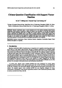
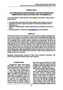
2 begin ,2 begin + stepsize...2 end . Specifying “-v n” indicates that we wish to do n-fold cross validation (in the above command n = 10), and the last argument to the command indicates which data file to use. The output of the program is a contour plot, saved in an image file of the name rescaled_training_data_file.png. The output image for the above command is depicted in Figure 6.
Figure 6: A contour plot of cross-validation accuracy for a given training set as produced by grid.py The contour plot indicates with various line colours the cross-validation accuracy of the classifier, as a function of C and σ – this is measured as a percentage of correct classifications, so that we prefer large values. Note that σ is in fact referred to as “gamma” by the libSVM software – the variable name is of course arbitrary, but we choose to refer to it as σ for compatibility with the majority of SVM literature. Given such a contour plot of performance, as stated previously there are generally two conclusions to be reached: 1. 2.
The optimal (or at least satisfactory) values of C and σ are contained within the plotting region. It is necessary to continue the search for C and σ, over a different range than that of the plot, in order to achieve better performance.
In the first case, we can read the optimal values of C and σ from the output of the program on the command window. Each line of output indicates the best parameters that have been encountered up to that point, and so we can take the last line as our operating parameters. In the second case, we must choose which direction to continue the search. From figure 6 it seems feasible to keep searching over a range of smaller σ and larger C. This whole procedure is usually quite effective, however there can be no denying that the search for the correct parameters is still something of a black art. Given this, we invite interested readers to experiment for themselves, in order to get a basic feel for how things behave. For our purposes, we shall assume that a good choice is C = 2-2 = 0.25 and σ = 2-2 = 0.25, and proceed to the next step. Training (svm-train) As we have seen, the cross validation process does not use all of the data for training – at each iteration some of the training data must be excluded for evaluation purposes. For this reason it is still necessary to do a final training run on the entire training set, using the parameters that we have determined in the previous parameter selection process. The command to train is: svm-train –g 0.25 –c 0.25 rescaled_training_data_file model_file This command sets C and σ using the –c and –g switches, respectively. The other two arguments are the name of the training data, and finally the file name for the learnt decision function or model.
Prediction (svm-predict) The final step is very simple. Now that we have a decision function, stored in the file model_file as well as a properly scaled set of unlabelled data, we can compute the predicted label of each of the examples in the set of unlabelled data by executing the command: svm-predict rescaled_unlabelled_data_file model_file predictions_file After executing this command, we will have a new file of the name predictions_file, Each line of this file will contain either “+1” or “-1” depending on the predicted label of the corresponding entry in the file rescaled_unlabelled_data.
Summary The general problem of induction is an important one, and can add a great deal of value to large corporate databases. Analysing this data is not always simple however, and it is fortunate that methods that are both easy to apply and effective have finally arisen, such as the Support Vector Machine. The basic concept underlying the Support Vector Machine is quite simple and intuitive, and involves separating our two classes of data from one another using a linear function that is the maximum possible distance from the data. This basic idea becomes a powerful learning algorithm, when one overcomes the issue of linear separability (by allowing margin errors), and implicit mapping to more descriptive feature spaces (through the use of kernel functions). Moreover, there exist free and easy to use software packages, such as libSVM, that allow one to obtain good results with a minimum of effort. The continued uptake of these tools is inevitable, but is often impeded by the poor results obtained by novices. We hope that this chapter is a useful aid in avoiding this problem, as it quickly affords a basic understanding of both the theory and practice of the SVM.
References Bishop, C. (1995), Neural Networks for Pattern Recognition, Oxford University Press. C.-W. Hsu, C.-C. Chang, C.-J. Lin (2003). A practical guide to support vector classification. Available at http://www.csie.ntu.edu.tw/~cjlin/papers/guide/guide.pdf K-W Cheung, J. T. Kwok, M. H. Law and K-C Tsui (2003), Mining customer product ratings for personalized marketing, Decision Support Systems pp 231-243. Chih-Chung Chang and Chih-Jen Lin (2001), LIBSVM : a library for support vector machines. Software available at http://www.csie.ntu.edu.tw/~cjlin/libsvm DeCoste, D. & Schölkopf, B (2002), Training Invariant Support Vector Machines. Machine Learning pp 161-290. Duda, R.O., Hart, P.E., Stork, D.G.(2001). Pattern Classification. John Wiley and Sons Inc. Hand, D. J. (1981), Discrimination and Classification, John Wiley and Sons Inc. Joachims, T. (2002b). SVMlight (Version 5.0). Joachims, T (2002), Learning to Classify Text Using Support Vector Machines: Methods, Theory and Algorithms, Kluwer Academic Publishers. Platt, J. (1999). Sequential Minimal Optimization: A Fast Algorithm for Training Support Vector Machines. In B. Schölkopf, C. J. C. Burges & A. J. Smola (Eds.), Advances in Kernel Methods - Support Vector Learning (pp. 185-208): MIT Press. Popper, K.R. (1968), The Logic of Scientific Discovery. Hutchinson. Quinlan, R. (1993, C4.5: Programs for Machine Learning, Morgan Kaufmann Publishers Inc. Rosenblatt, F. (1958). The Perceptron: A Probabilistic Model for Information Storage and Organization in the Brain. In Psychological Review, Volume 65, November, 1958, pp. 386-408. Sansom, D. C. and Downs, T. and Saha, T. K. (2002), Evaluation Of Support Vector Machine Based Forecasting Tool In Electricity Price Forecasting For Australian National Electricity Market Participants. In Australasian Universities Power Engineering Conference. Schölkopf, B., & Smola, A. (2002). Learning with Kernels: Support Vector Machines, Regularization, Optimization, and Beyond. Cambridge, MA: MIT Press. Weiss, S. A.. & Kulikowski, C. A. (1991), Computer Systems That Learn: Classification and Prediction Methods from Statistics, Neural Nets, Machine Learning, and Expert Systems, Morgan Kaufmann. Vapnik, V. N. (1998). Statistical Learning Theory. New York: Wiley. Zan Huang and Hsinchun Chen and Chia-Jung Hsu and Wun-Hwa Chen and Soushan Wu (2004), Credit Rating Analysis with Support Vector Machines and Neural Networks: a market comparitive study, Decision Support Systems pp543-558.