*Department of Radiology, University of Chicago. 5841 South Maryland Avenue, Chicago, IL 60637 ... the first time the use of support vector machine (SVM).
SUPPORT VECTOR MACHINE LEARNING FOR DETECTION OF MICROCALCIFICATIONS IN MAMMOGRAMS1 �
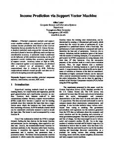
Issam El-Naqa, Yongyi Yang, Miles N. Wernick, Nikolas P. Galatsanos, and Robert Nishikawa* Dept. of Electrical and Computer Engineering, Illinois Institute of Technology 3301 S. Dearborn Street, Chicago, IL 60616 *Department of Radiology, University of Chicago 5841 South Maryland Avenue, Chicago, IL 60637 ABSTRACT Microcalcification (MC) clusters in mammograms can be an indicator of breast cancer. In this work we propose for the first time the use of support vector machine (SVM) learning for automated detection of MCs in digitized mammograms. In the proposed framework, MC detection is formulated as a supervised-learning problem and the method of SVM is employed to develop the detection algorithm. The proposed method is developed and evaluated using a database of 76 mammograms containing 1120 MCs. To evaluate detection performance, free-response receiver operating characteristic (FROC) curves are used. Experimental results demonstrate that, when compared to several other existing methods, the proposed SVM framework offers the best performance. 1. INTRODUCTION Microcalcification (MC) clusters are an indicator of breast cancer, which is a leading cause of death in women. MCs are tiny calcium deposits that appear as small bright spots in a mammogram (as illustrated in Fig. 1). Individual MCs are sometimes difficult to detect because of the surrounding breast tissue, their variation in shape, orientation, brightness and size (typically, 0.05-1mm) [1]. In the literature, a great many image-processing methods have been proposed to detect MCs automatically. Here, we briefly cite a few. A statistical Bayesian image analysis model was developed in [2]. A difference image technique was investigated in [3]. Wavelet based approaches were studied in [4]. A detection scheme using multi-scale analysis was proposed in [5]. Methods based on weighted difference of Gaussian filtering were used in [6]. A method based on higher-order statistics was developed in [7]. A fuzzy logic approach was proposed in [8]. A 2D adaptive lattice algorithm was used to predict correlated clutters in the mammogram in [9]. Fractal 1
This work was supported in part by NIH/NCI grant CA89668.
modeling was proposed in [10]. A method based on “region growing” and active contours was studied in [11]. More recently, a two-stage neural network approach was proposed in [12]. In this work we investigate for the first time the use of a support vector machine (SVM) learning framework for MC detection, and show that it provides the best performance among the methods we have tested so far. SVM learning is based on the principle of structural risk minimization [13]. Instead of directly minimizing learning error, it aims to minimize the bound on the generalization error. As a result, an SVM is able to perform well when applied to data outside the training set. In recent years SVM learning has been applied to a wide range of realworld applications where it has been found to offer superior performance to that of competing methods [14]. In the proposed work, MC detection is considered as a two-class pattern classification task performed at each location in the mammogram. The two classes are “MC present” and “MC absent.” With an SVM formulation, a nonlinear classifier is trained using supervised learning to automatically detect the presence of MCs in a mammogram.
Figure 1. A section of a mammogram containing multiple MCs (labeled with circles).
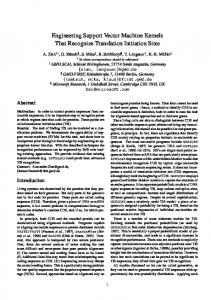
2. METHODOLOGY 2.1. SVM classifier The basic idea of an SVM classifier is illustrated in Fig. 2. This figure shows the simplest case in which the data vectors (marked by ‘X’s and ‘O’s) can be separated by a hyperplane. In such a case there may exist many separating hyperplanes. Among them, the SVM classifier seeks the separating hyperplane that produces the largest separation margin [13,14]. Such a scheme is known to be associated with structural risk minimization [13]. In the more general case in which the data points are not linearly separable in the input space, a nonlinear transformation is used to map the data vector x into a high-dimensional space (called feature space) prior to applying the linear maximum-margin classifier. To avoid the potential pitfall of over-fitting in this higherdimensional space, an SVM uses a kernel function in which the nonlinear mapping is implicitly embedded. According to Cover’s theorem [13], a function qualifies as a kernel provided that it satisfies the Mercer’s conditions. With the use of a kernel, the discriminant function in an SVM classifier has the following form: LS
g ( x) = ∑ α i d i K ( xi , x) + α o ,
(1)
i =1
where K (⋅, ⋅) is the kernel function, x i are so-called support vectors determined from training data, LS is the number of support vectors, di is the class indicator (e.g., +1 for class 1 and –1 for class 2) associated with each x i , and αi are constants, also determined from training. By definition, support vectors (Fig. 2) are elements of the training set that lie either exactly on or inside the decision boundaries of the classifier. In essence, they consist of those training examples that are most difficult to classify. The SVM classifier uses these “borderline” examples to define its decision boundary between the two classes. This in philosophy is quite different from a classifier that is based on minimizing leaning error alone. Note that in a typical SVM learning problem only a small portion of the training examples will typically qualify as support vectors. 2.2. Design of SVM Classifier for MC Detection A. Input feature vector MCs appear as tiny bright spots in a mammogram. To test the presence of an MC at a given location, we use as input pattern to the SVM the pixel values in a small M × M window centered at that location. We chose M=9 to accommodate the MCs, the average size of which was around 6-7 pixels in diameter in our data set. Such a window size can effectively avoid any potential interference from neighboring MCs.
Figure 2. Support vector machine classification with a linear hyperplane that maximizes the separating margin between the two classes. Alternatively, other image features (e.g., local edges, etc.) might prove more salient rather than pixel values for the input pattern. However, it is not clear what defines the complete set of salient features deemed relevant for MC detection. Thus, we used image pixels. The image must be preprocessed before the pixel values are used. A high-pass filter with a very narrow stop-band was applied to mitigate the effect of spatial inhomogeneity of the background. This filter was designed as a length-41, linear-phase FIR filter with cutoff frequency wc=0.125. B. SVM kernel functions The kernel function plays the central role of implicitly mapping the input vector into a high-dimensional feature space, in which better separability is achieved. In this study the following two types of kernel functions are considered: 1. Polynomial kernel
K (x, y ) = (xT y + 1) p , where p > 0 is a constant . 2. Gaussian radial basis function (RBF) kernel x−y 2 , K (x, y ) = exp − 2σ 2 where σ > 0 is a constant that defines the kernel width. Both of these kernels satisfy the Mercer’s conditions [13], and are among the most commonly used in SVM. C. Training examples Training examples are gathered from the mammograms as follows: for the “MC present” class (designated Class 1), image windows of size M × M are collected at the centers of mass of the MCs identified in the database; for the “MC absent” class (designated Class 2), image windows are collected from those regions of the image containing no MCs. Because there are typically far more background regions than regions containing MCs, a
D. SVM training Let x i denote the input feature vector for each of the training set elements. Then the desired response of the classifier di = +1 if x i belongs to Class 1 and di = −1 if x i belongs to Class 2. The support vectors and other parameters in the decision function g(x) in (1) are determined through numerical optimization during the training phase. Specifically, the dual form of the optimization problem for maximal margin separation is given as: N G 1 N N min J (α ) = ∑ α i − ∑∑ α iα j di d j K (xi , x j ) , (2) 2 i =1 j =1 i =1 subject to the following constraints: l
(1)
∑α d i =1
i
i
= 0; and
(2) 0 ≤ α i ≤ C for i = 1, 2,..., N , where N is the total number of training samples, C is a positive regularization parameter that controls the tradeoff between complexity of the machine and the allowed classification error. It is noted that the number of training samples used in this study is rather large (on the order of several thousands). Traditional optimization algorithms can no longer be efficiently applied in this case. Fortunately, more efficient algorithms have been developed in recent years for the SVM optimization problem [14]. These algorithms typically take advantage of the fact that the Lagrange multipliers in (2) are mostly zeros. In this study, a technique called successive minimal optimization [15] is adopted. E. SVM model selection During the training phase, the following variables need to be determined for the SVM classifier: the kernel function to use, and the regularization parameter C. For this purpose, we adopt a widely used statistical method called m -fold cross-validation, which consists of the following steps: 1) divide randomly all the available training examples into m equal-sized subsets; 2) use all but one subset to train the SVM; 3) use the held out subset to measure classification error; 4) repeat Steps 2 and 3 for each subset, 5) average the results to get an estimate of the generalization error of the SVM classifier. The SVM was tested using this procedure for various parameter settings. In the end, the model with the smallest generalization error was adopted.
3. EXPERIMENTAL RESULTS 3.1. Data set The proposed algorithm was developed and evaluated using a data set provided by the Department of Radiology at the University of Chicago. This data set consists of 76 mammograms, digitized with a spatial resolution of 0.1 mm/pixel and 10-bit grayscale. In the data set, 1120 individual MCs were identified by experienced mammographers. In this work, the mammograms in this data set were divided equally into two subsets in a random fashion, one used exclusively for training (designated training mammogram set), and the other exclusively for testing (designated test mammogram set). 3.2. Training and model selection results The examples used for SVM training include a total of 547 for Class 1, and twice as many for Class 2. Such a choice is a result of compromise between the vast number of available Class-2 examples and the complexity of the training. The SVM classifier was then trained using a 10-fold cross-validation procedure for various model and parametric settings. In Fig. 3 we show a plot of the estimated generalization error rate for the trained SVM classifier with the Gaussian RBF kernel. A generalization level as low as 6% was achieved under various parametric settings. These results demonstrate that the performance of the SVM classifier is rather robust over the choice of model parameters. Interestingly, similar error level was also achieved when the polynomial kernel with p=3 was used. Due to space limitation these results are not shown. In the evaluation study below, the SVM classifier using the Gaussian RBF kernel with σ = 5 and C = 1000 was σ=2.5 σ=5 σ=10
0.25 0.2 Misclassification rate
random sampling scheme is adopted for Class-2 examples so that the training examples are representative of all the mammograms.
0.15
0.1 0.08
0.06 0.05 -1 10
0
10
1
10
2
10 C
3
10
4
10
5
10
Figure 3. Plot of generalization errors versus the regularization parameter C , achieved by the SVM classifier using the Gaussian RBF kernel with σ = 2.5, 5, and 10.
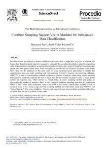
used. The number of resulting support vectors for this case was about 12% of the total number of training samples; the training time was about 7 seconds (implemented in MATLAB on a Pentium III 933 MHz dual-processor PC). 3.3. Other methods for comparison The proposed algorithm was compared with four other existing methods for MC detection: (1) the image difference technique (IDT) in [3]; (2) the difference of Gaussians (DoG) method in [6]; (3) the wavelet based method in [4]; and (4) the two-stage multi-layer neural network method in [12]. In our implementation, these methods were typically run for numerous parameter settings and the one yielding the best result was chosen for the final evaluation. 3.4. Evaluation Results The detection performance was evaluated quantitatively using the free-response receiver operating characteristic (FROC) curves [16]. An FROC curve plots the correct detection rate (i.e., true-positive fraction) versus the average number of false-alarms (i.e., false-positives) per image for the continuum of the decision threshold. The FROC curve provides a comprehensive summary of the trade-off between missed detections and false alarms. All the detection algorithms were evaluated using the same set of 38 test mammograms. The results are summarized using FROC curves in Fig. 4. As can be seen, the SVM classifier offers the best result in the operating range with less than 3 false clusters per image. The small section shown in Fig. 1 was from a test mammogram containing several MCs; these MCs (though some of them are hardly visible) were all successfully detected by the SVM classifier and labeled with circles. 1
0.9
TP fraction
0.8
0.7
0.6 SVM Classifier Wavelet DoG IDTF Neural Network
0.5
0.4 0
1
2 3 Avg. Number of False Clusters
4
5
Figure 4. FROC curves obtained for the different methods evaluated. A higher FROC curve indicates better performance. The most significant portion of the curves is at the low end of the number of false positive clusters, where one would prefer to operate.
4. CONCLUSTIONS In this work we demonstrated an SVM based classifier to detect microcalcifications in mammogram images. Experimental results show that the proposed framework is quite robust over the choice of several model parameters. In these initial results the SVM classifier outperformed all the other methods considered. 5. REFERENCES [1] M Lanyi, Diagnosis and Differential Diagnosis of Breast Calcifications, Springer-Verlag, Berlin, 1988. [2] N. Karssemeijer, “A stochastic model for automated detection calcifications in digital mammograms,” in Proc. 12th Int. conf. Info. Med. Imag., Wye, UK, July 1991. [3] R. M. Nishikawa, et al, “Computer aided detection of clustered Microcalcifications in digital mammograms,” Med. Bio Eng. Comp., vol. 33, 1995. [4] R. N. Strickland, and H. L. Hahn, “Wavelet transforms methods for object detection and recovery”, IEEE Trans. Image Processing, vol. 6, pp. 724-735, May 1997. [5] T. Netsch, “A scale-space approach for the detection of clustered microcalcifications in digital mammograms,” 3rd Int. Workshop on Digital Mammography, 1996. [6] J. Dengler, S. Behrens, and J.F. Desaga, “Segmentation of microcalcifications in mammograms,” IEEE Trans. Med. Imag., vol. 12 no. 4, 1993. [7] M. N. Gurcan, et al, “Detection of microcalcifications in mammograms using higher order statistics,” IEEE Signal Proc. Lett., vol. 4, no. 8, 1997. [8] H. Cheng, Y. M. Lui, and R. I. Freimanis, “A novel approach to microcalcifications detection using fuzzy logic techniques,” IEEE Trans. Med. Imag., vol. 17 no. 3, June 1998. [9] P. A. Pfrench, J. R. Zeidler, and W.H. Ku, “Enhanced detectability of small objects in correlated clutter using an improved 2-D adaptive lattice algorithm”, IEEE Trans. Imag. Proc., vol. 6 no. 3, 1997. [10] H. Li, K. J. Liu, and S. B. Lo, “Fractal modeling and segmentation for the enhancement of microcalcifications in digital mammograms,“ IEEE Trans. Med. Imag., vol. 16, no. 6, Dec. 1997 [11] I. N. Bankman, et al, “Segmentation algorithms for detecting microcalcifications in mammograms,” IEEE Trans. Info. Tech. in Biomed., vol. 1, no. 2, June 1997. [12] S. Yu, and L. Guan, “A CAD system for the automatic detection of clustered microcalcifications in digitized mammogram films,” IEEE Trans. Med. Imag., vol. 19, pp. 115126, Feb. 2000. [13] V. Vapnik, Statistical Learning Theory, Wiley, 1998. [14] K. R. Muller, S. Mika, G. Ratsch, K. Tsuda, and B. Scholkopf, “An introduction to kernel-based learning algorithms,” IEEE Trans. Neural Networks, vol. 12, no. 2, pp.181-201, 2001. [15] J. Platt, “Fast training of support vector machine using sequential minimal optimization”, Advances in Kernel Methods: Support Vector Learning, ed., Scholkopf et al, MIT Press, 1998. [16] P. C. Bunch, et al, “A free-response approach to the measurement and characterization of radiographic-observer performance”, J. Appl. Eng. vol. 4, 1978.