An inversion algorithm for retrieval of aerosol optical ...

An inversion algorithm for retrieval of aerosol optical and physical properties from ground-based solar and sky radiance Qie Lili1,2, Xu Qingshan1, and Wei Heli1 (1 Key Laboratory of Atmospheric Composition and Optical Radiation, Anhui Institute of Optics and Fine Mechanics, the Chinese Academy of Sciences, P.O. Box 1125, Hefei, Anhui 230031, China) (2 Graduate University Chinese Academy of Sciences, Beijing, China, 100049)

ABSTRACT An inversion algorithm has been developed for retrieving a set of parameters of aerosol scattering and microphysical properties from POM02 sky-radiometer measurements. POM01/02 is the main observation instrument of Skynet. It’s designed to measure solar and sky irradiance with waveband ranging from visible to infrared, as well as the measurement of polarization sky radiance at 870nm wavelength. Teruyuki Nakajima developed a software package to analyze its observation data named SKYRAD.pack. SKYRAD.pack code can retrieve the columnar aerosol features, such as optical depth, single-scattering albedo, phase function and size distribution, provided the input parameters, such as complex refractive index and ground albedo, are correctly given. In our algorithm, most of aerosol key characteristics, including single-scattering albedo, phase function, polarized phase function at 870nm, complex refractive index, and size distribution, are retrieved from direct and scattered solar irradiance as well as polarized sky radiance at 870nm, by using a polarized radiative transfer code RT3. This method requires only measurement of the aerosol’s optical thickness and an estimate of the ground’s reflectance and does not need any specific assumption about properties of the aerosol. The preliminary results are reported in the paper. Aerosol property; Polarization; Retrieval algorithm.

1

INTRODUCTION

Atmospheric aerosol affects climate and environment in complex ways. Many uncertainties remain in understanding aerosol forcing of the climate system, because of its great temporal and spatial variability. The parameters of aerosol information on a global scale are essential for reducing these uncertainties. Various ground-based and space-borne observation systems have been developed to provide aerosol properties, e.g. ground-based sun-photometer networks (AERONET, SKYNET) and satellite instruments (POLDER, MODIS, MISR). Long-term ground-based network is extremely important as it is vital for satellite validation, model evaluation, and climate change assessment from trend analysis. Inversion procedure is the core part of remote sensing, whereby aerosol optical and physical properties are derived from the remote sensing measurements. Over the past decades, a number of inversion methods have been proposed for interpreting the ground-based radiative measurements of the cloud-free atmosphere. For example, the method of King et al.[1] retrieved the particle size distribution by using spectral aerosol optical thickness only, while Nakajima et al.[2,3] used angular distribution of sky radiance, and Dubovik and King’s algorithm[4,5] for AERONET including a detailed statistical optimization of the influence of noise. Multiple-scattering effects were adequately accounts for in the whole range of the International Symposium on Photoelectronic Detection and Imaging 2011: Advances in Infrared Imaging and Applications, Jeffery J. Puschell, Junhao Chu, Haimei Gong, Jin Lu, Eds., Proc. of SPIE Vol. 8193, 81934C · © 2011 SPIE · CCC code: 0277-786X/11/$18 · doi: 10.1117/12.901090 Proc. of SPIE Vol. 8193 81934C-1 Downloaded from SPIE Digital Library on 29 Nov 2011 to 211.86.158.134. Terms of Use: http://spiedl.org/terms

scattering angles by Nakajima et al.[3], which is required especially at large scattering angles. This was an important improvement. Wendisch and Hoyningen-Huene[6,7] extended the scattering angles to almucantar of the Sun to estimate the aerosol refractive index, and emphasized the usefulness of extending sky radiance measurements to larger scattering angles. Wang and Gordon[8] derived aerosol phase function and the single-scattering albedo from direct and sky radiance over the ocean. With the contributions of ground reflection precisely corrected, Devaux et al.[9] extended Wang and Gordon’s algorithm over ground surface. Because the polarization measurements add more useful information to the retrieval of aerosol microphysical properties, Vermeulen et.al.[10] and Li et.al.[11] proposed that the polarized phase function, the aerosol size distribution and refractive index can be retrieved by adding the sky polarized radiance measurement. POM01/02 sky-radiometer is the main observation instrument of Skynet. It’s designed to measure sun and sky irradiance covering wavelength from visible to infrared, as well as the polarization measurement of sky radiance in 870nm. Its observation data can be analyzed using Skyrad.pack developed by Nakajima et.al.[3], but the polarized radiance was not considered. Thus, we developed a scheme for retrieval of aerosol characteristics. In our algorithm, the polarized radiative transfer code RT3[12] is implemented, in which the adding-doubling method was used to compute multiple-scattering of aerosol. Most of aerosol properties were retrieved by the algorithm, including single scattering albedo, phase function, polarized phase function, size distribution, and complex refractive index.

2

Methodology

We intend to retrieve the aerosol single-scattering albedo

ω0 , and the scattering phase function pa ( the P11 (θ )

in the scattering phase matrix) and polarized phase function qa ( the P12 (θ ) in the scattering phase matrix) from measurements of the direct solar radiance and scanning of the scattered sky radiance in the solar principal plane (SPP). The method has been detailed by Devaux et al.[9] and Vermeulen et al.[10]. It consists of retrieving ω0 . The direct solar radiation extinction, after the correction of Rayleigh scattering and gaseous absorption, provides the aerosol optical thickness for extinction,

τ a . On the other hand, the scattered sky radiance, after the elimination of the contributions of

ground reflection, Rayleigh and multiple-scattering, may provide the radiance singly scattered by aerosols, from which the aerosol optical thickness for scattering the aerosol single-scattering albedo

τs

can be derived by the integral 2π

ω 0 = τ s / τ a is obtained. Once ω0

is known,

∫

π

0

La1 (θ ) ,

La1 (θ ) sin θ dθ . Thus

pa and qa can be derived from

total and polarized sky radiances by radiative transfer calculation with the code RT3. As aerosol’s optical properties are dominated by its physical properties, finally, one can use the modified constrained linear inversion method to retrieve aerosol microphysical properties[1,10,11]. 2.1 Retrieval of optical properties of atmospheric aerosol The method of Devaux et al.[9] are used here. We set

ω0*

and

pa* as the initial guess for the aerosol

Proc. of SPIE Vol. 8193 81934C-2 Downloaded from SPIE Digital Library on 29 Nov 2011 to 211.86.158.134. Terms of Use: http://spiedl.org/terms

single-scattering albedo and phase function, and

ρ g*

as the estimated ground reflectance. We can simulate the

estimated total sky radiance L (τ a , ω 0 , pa , ρ g ) and that corresponding black surface, L 0 (τ a , ω 0 , pa , 0) . Then *

*

*

*

*

the ground contribution in the measurements is approximately, parameters

ω0*

and pa

*

*

*

ΔL ≈ ΔL* = L* − L0* . Provided that the guessed

are close to the real value, then the ratios (single scattering/total scattering) will be nearly

the same for calculation and measurement. That is,

(ω0*τ a pa* + τ m pm ) / 4 cos θ v (ω0τ a pa + τ m pm ) / 4 cos θ v = . L0* L − ΔL*

θv

Where L is the actual total sky radiance,

is view zenith angle,

τm

(1)

and pm denotes Rayleigh scattering optical

thickness and phase function, respectively. With a simple transformation,

ω0 pa L − ΔL* * L − L* τ m = pa + pm . L0* L0* ω0*τ a ω0*

(2)

and the phase function normalization yields,

∫

π

0

θ

Where，the

ω0 *

ω0

(3)

is scattering angle. By substituting (2) in (3), we obtain

2ω0

Obviously, if

pa (θ , λ ) sin θ dθ = 2 .

ω0*

π

=∫ [ 0

L − ΔL* * L − L* τ m pa + pm ]sin θ dθ . L0* L0* ω0*τ a

equal to the true single-scattering albedo *

can be deduced. We recalculate L and L0

*

(4)

ω0 , the integral result on the right should be 2. Then the

corresponding to the real albedo

ω0

by running radiative transfer

code RT3, and substitute them into Eq.(2), pa will be retrieved. A similar scheme is applied to the polarized sky radiance L p to retrieve the polarized phase function qa . There is no need for correction of ground contamination, due to the influence of the ground reflectance on the polarized sky radiance is negligible[10].

L p − L* p (ω0 ) τ m qa = * qa + qm . Lp (ω0 ) L p* (ω0 ) ω0τ a Lp

Here, qa

*

*

(5)

and qm denote initial guess of polarized phase function and Rayleigh scattering polarized phase function,

Proc. of SPIE Vol. 8193 81934C-3 Downloaded from SPIE Digital Library on 29 Nov 2011 to 211.86.158.134. Terms of Use: http://spiedl.org/terms

respectively. L p (ω0 ) is the calculated polarized sky radiance. *

2.2 Retrieval of physical properties of atmospheric aerosol King et al.[1] and Vermeulen et al.[10] had discussed the retrieval of aerosol size distribution from spectral optical thickness

τ a (λ )

or phase function pa (θ ) , separately. Li et al.[11] pointed out that introducing more information into

the retrieval kernel function is valuable, they implemented the conjoint using of

τa

and pa in their retrieval, called

modified constrained linear inversion method. We assume that the aerosol is consisted of spherical homogeneous particles,

τ a (λ ) = ∫

rmax

rmax

rmin

Where

and pa are given by the integral

f (r )[π r 2Qe (r , λ , m)h(r )]dr .

rmin

Pa (θ ) = C ∫

τa

f (r )[π r 2Qs (r , m, λ ) P (θ , r , m, λ )h(r )]dr .

(6) (7)

Qe (r , λ , m) is the extinction efficiency factor calculated from Mie theory, while Qs (r , m, λ ) is the

scattering efficiency factor, and

P (θ , r , m, λ ) is the normalized phase function of a particle with radius r and

refractive index m at the wavelength

λ . rmin

and

rmax are the lower and upper limits of r . The size distribution

n(r ) has been replaced by f (r )h(r ) , where f (r ) is a slowly varying function of r , while h(r ) is rapidly varying and usually takes the form of a Junge size distribution

r − (α +3) as initial guess, α is Angstrom exponent. C

is a constant and yields,

1 = C∫

rmax

rmin

We assume that

τa

Qs (r , λi , m)n(r )dr .

are measured at N wavelengths and

(8)

pa are retrieved at M angles. The integral in Eq.(6), (7)

is replaced by a summation over several intervals in r . Following King et al.[1], Eq.(6), (7) are written as the matrix of linear equations

g = Af + ε .

εi

where

ε

∑A

f j . The other elements of (9) are given by

ij

is error vector whose elements

(9)

represent the deviation between measurement gi and calculation

j

Proc. of SPIE Vol. 8193 81934C-4 Downloaded from SPIE Digital Library on 29 Nov 2011 to 211.86.158.134. Terms of Use: http://spiedl.org/terms

⎧τ a (λi ), i = 1, N . gi = ⎨ ⎩ pa (θi ), i = N + 1, N + M

(10)

⎧ rj+1 π r 2Q (r , λ , m)h(r )dr , i = 1, N e i ⎪ ∫rj Aij = ⎨ r j +1 ⎪ ∫ π r 2Qs (r , λ , m) P (θi , r , m, λ )h(r )dr , i = N + 1, N + M . r j ⎩

(11)

The solution of Eq.(9) was derived by Twomey[13], the solution of least square method with quadratic constraints, given by

f = ( AT C −1 A + γ H ) −1 AT C −1 g . Where

γ

is some non-negative Lagrange multiplier,

(12)

H is the smoothing matrix, C is measured covariance matrix,

gives a relative weighting to each of the measurements. Here, we assume the same statistical errors for The fitness of retrieved

τa

and pa .

n(r ) for measurements is weighed by the rms residual

σg =

1 N +M

N +M

∑ i =1

2

⎛ εi ⎞ ⎜ ⎟ . ⎝ gi ⎠

We improve the retrieval scheme to derive a stable result of

(13)

n(r ) by reloading the retrieved n(r ) as the

improved h( r ) , the convergence toward a solution requires that each element of

f converges to unity. The selected

scattering angles and classes of particle radius have to be optimized, and the upper and lower limits of r have to be adjusted according to aerosol type, otherwise instabilities might appear. To show how does the particles at radius r contribute to the phase function at arbitrary scattering angle function as below, for a given size distribution

wp (r ,θ ) = Fig.1 illustrates the variations of

θ,

we define an phase function contribution weighting

n( r ) , C π r 3Qs (r , m, λ ) P(θ , r , m, λ )n(r ) . Pa (θ )

(14)

wp as a function of r and θ for three aerosol models (see section 3 for details). It

shows that particles smaller than 0.5μm contribute the most to the phase function at large scattering angles, while large particles, above 1.0μm contribute more to small angles, particles smaller than 0.04 μm have teeny contribution to And it depends on aerosol model in detail. Also it is important to select an appropriate value for

Proc. of SPIE Vol. 8193 81934C-5 Downloaded from SPIE Digital Library on 29 Nov 2011 to 211.86.158.134. Terms of Use: http://spiedl.org/terms

γ

pa .

, so that all elements

of the solution vector variation of

f are positive, and σ g is small[14]. It is also required that σ g does not oscillate with minor

γ , as it’s obvious that a stable solution of n(r )

an example of the rms residual

σg

as a function of

γ . σg

For a given refractive index m , the best solution of

oscillates up and down when

γ

γ . Fig.2 Shows

is small.

n(r ) indicated by σ g is derived, but no information about

the aerosol refractive index can be obtained from the indicator both

should not affected by a perturbation to

σ g . Thus，

another indicator σ q , which is sensitive to

n(r ) and m , is combined with to determine this two physical properties simultaneously. σ q is given by

σq = Where

1 M

2

⎛ q cal (θi ) − q (θi ) ⎞ ⎜ ⎟ . ∑ q(θi ) i =1 ⎝ ⎠ M

(15)

q cal (θi ) denotes the retrieved qa corresponding to the given m and the retrieved n(r ) . Which is

calculated by Mie theory .

Proc. of SPIE Vol. 8193 81934C-6 Downloaded from SPIE Digital Library on 29 Nov 2011 to 211.86.158.134. Terms of Use: http://spiedl.org/terms

Fig.1 The variations of aerosol phase function contribution weighting function as a function of aerosol radius and scattering angles for three aerosol models: (a)Water-Soluble (b)Dust, and (c) Biomass Burning aerosol.

σg

1E-3

1E-4

1E-5 1E-3

0.01

0.1

1

10

100

γ

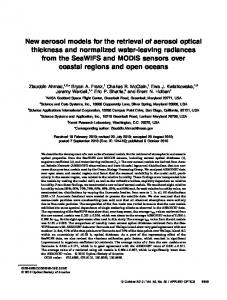
Fig.2 An example of the rms residual between g and Af as a function of Lagrange multiplier. The rms residual oscillates when is small.

3

Validation of the method

We assess the algorithm performance by numerical experiments. Obviously, the retrieval accuracy may be different for different aerosol types because the relationships between measurements and retrieved properties are complex and nonlinear. Three typical aerosol models are considered here, i.e, water-soluble, dust, and biomass burning aerosol models. These models were also used by Dubovik et al.[5] and Li et al.[11] to validate their algorithms theoretically. The model is described as the sum of two log-normal distribution functions 2 (ln r − ln rmean ,i ) Ci dN =∑ exp[− ], 2σ i 2 dr i =1 2πσ i r 2

the parameters for the three models are listed in Tab.1.

Proc. of SPIE Vol. 8193 81934C-7 Downloaded from SPIE Digital Library on 29 Nov 2011 to 211.86.158.134. Terms of Use: http://spiedl.org/terms

(16)

Table 1. The bimodal log-normal aerosol model parameters used in the theoretical validation

Aerosol type Water-soluble Dust Biomass burning 3.1

σ1

σ2

rmean,1(μm)

rmean,2(μm)

C1/C2

mr+imi

0.6 0.6 0.4

0.6 0.8 0.6

0.04 0.034 0.082

0.4 0.5 1.52

2000 735 65700

1.45-i0.004 1.53-i0.008 1.52-i0.025

Retrieval of optical properties

Firstly, the model aerosol optical properties are computed by Mie theory. The optical properties include

τ a (λ ) , ω0 ,

pa , and qa , particle radius ranging from 0.01 to 10 μm. Then we input these parameters into the RT3 code, to simulate the total and polarized radiance in SPP at 870nm, assuming that solar zenith angle, reflectance, ρ g

θ 0 = 60°

, ground

= 0.2 , τ a = 0.4 , and τ m = 0.015 . The calculated L and L p at 26 scattering angles ranging from

6°to 147°are used as simulated measurements for retrieval. We choose a Junge aerosol model as the initial guess, for which the Angstrom exponent is estimated from the spectral optical thickness

τ a (λ ) , and the refractive index is the

same as model aerosol. To derive ω0 , a simple interpolation is used. We calculate the integral on the right hand of Eq.(4) for several

ω0*

from 0.5 to 1.0, then we interpolate the obtained integral values, find the

ω0*

corresponding to 2. It

should be noted that at the missing measurements scattering angle, we substitute the integral kernel by The results are shown in Fig.3 and are summarized in Tab.2. The retrieved

* pa（ θ）.

pa and qa for biomass burning model

departs significantly from the true phase function. So we tried another initial guess, the initial guess Junge model for water-soluble model, who’s

pa* towards to the true pa more close at the forward-scattering angles. That may be

important for the retrieval algorithm, because the spike at small scattering angle of aerosol phase function. We found that the accuracy improved at the second retrieval. Thus the retrieved

pa and qa rely a bit on the initial guess pa* . It

suggests that an iterative procedure improve the results, by setting the retrieved algorithm again and again until a stable

pa as a new guess, runing the

pa and qa is derived.

Proc. of SPIE Vol. 8193 81934C-8 Downloaded from SPIE Digital Library on 29 Nov 2011 to 211.86.158.134. Terms of Use: http://spiedl.org/terms

0.10

Ture Initial guess Retrived

10

0.05 0.00

P11

P12

-0.05 -0.10

1

-0.15 -0.20

Water-solubal

Water-solubal

0.1

-0.25 0

20

40

60

80

100

120

140

160

180

0

20

40

o

60

80

100

120

140

160

180

o

scattering angle( )

scattering angle( ) 0.12

Dust

100

Dust

0.10 0.08 0.06

P11

P12

10

1

0.04 0.02 0.00

-0.02 -0.04

0.1

-0.06 0

20

40

60

80

100

120

140

160

180

0

20

40

o

60

80

100

120

140

160

180

o

scattering angle( )

scattering angle( ) 0.1

P11

10

0.0 -0.1

P12

True Inicial guess 1 retrieved 1 Inicial guess 2 retrieved 2

-0.2 -0.3

1

-0.4 -0.5

Biomass buring 0.1

Biomass buring

-0.6 0

20

40

60

80

100

120

140

160

180

0

20

o

Fig.3

40

60

80

100

120

140

160

180

o

scattering angle( )

scattering angle( )

Validation of aerosol optical properties retrieval scheme. The truths, the initial guesses and the retrievals of Pa, qa, for three

typical models, are presented simultaneously for comparison. For the Biomass burning model, retrieval is preformed twice. At the retrieval 2, the initial guess for Water-soluble model is used as initial guess. Table 2. The errors for retrieving three typical aerosol models

Error of average on retrieval of

Water-soluble

Dust

Biomass burning (retrieval 1)

Biomass burning (retrieval 2)

ω0

-0.89% 1.5%

-2.56% 8.4%

3.65% 33.8%

-2.35% 4.3%

0.006

0.007

0.114

0.026

No error No error

0.005 No error

Pa(6-147°) qa( 6-147°) mr mi

0.005 0.005

The errors for ω0, Pa are relative errors, while errors for qa, mr, and mi are absolute errors.

Proc. of SPIE Vol. 8193 81934C-9 Downloaded from SPIE Digital Library on 29 Nov 2011 to 211.86.158.134. Terms of Use: http://spiedl.org/terms

3.2 Retrieval of size distribution and refractive index First of all, let’s prove that it’s feasible to retrieve aerosol spectral optical thickness

n(r ) and m simultaneously. Assuming exact retrieval of

τ a (λ ) ( at the wavelengths 1050, 870, 780, 670, 610, 520, 400nm) and phase function

pa ( at one wavelength 870nm, 26 scattering angles ranging from 6-147°), we run the scheme described in section 2.2 with several given m , including the true refractive index. In particular, to prevent there being too many insignificant matrix elements

Aij in Eq.(9), the upper and lower limits of particle radius retrieved has been adjusted for different

aerosol types. They are 0.04-9.0, 0.06-10.0, and 0.04-8.0 μ m for Water-soluble, Dust, Biomass burning models, respectively, considering the behaviors of the phase function contribution weighting function varied with r , illustrated in Fig.1.

n(r ) is retrieved at 15 sizes of radius, and the sizes are equal interval at ln r scale.

The retrieved

n(r ) is normalized and illustrated in Fig4., also the qa corresponding to various pairs of n(r )

and m are calculated by Mie theory, they are compared with models. The rms residuals

σ q , between the true and

retrieved qa , are shown in Tab.3. It shows that, both for

n(r ) and qa , the best fit between model and retrieval yields

σq

listed in Tab.3 illustrates the sensitivity of polarization to m ,

the correct value of m . Also The large variation of and the smallest value of

σq

yields to the true value of m for all the three aerosol models. So it’s feasible to retrieve

n(r ) and m simultaneously by adding σ q as another indicator. Now we perform an iterative process with a series of mr and mi . mr varies from 1.35 to 1.65, with step 0.025. Ten mi values varies from 0.0 to 0.05, they are 0.0, 0.001, 0.002, 0.004, 0.006, 0.008, 0.01, 0.02, 0.03, and 0.05. is calculated for every retrieval to search for a best fit. The relative errors between true

ω0

and calculated value,

σq σω

0

is also calculated. They are shown in Fig.5. The meaning of X axis is the complex refractive index. The first two digitals of X axis (hundreds and tens digit) correspond to mr , the last digital correspond to mi . Its hundreds and tens digit plus 1 denotes the num of mr , while its units denotes the number of mi . For example, in the diagram of water-soluble model, the smallest

σq

correspond to x= 44, it means the 5th mi (.i.e. 0.004) and the 4th mr (i.e.1.45), thus, X=44

Proc. of SPIE Vol. 8193 81934C-10 Downloaded from SPIE Digital Library on 29 Nov 2011 to 211.86.158.134. Terms of Use: http://spiedl.org/terms

means m = 1.45 − i 0.004 , the correct value.

σω

0

shows extremely sensitivity to mi , its extreme value always

indicates the best mi . Then the retrieval process may be optimized. We can run the inversion at an arbitrary mr and a series of mi , and search for the best two or three mi values, then run the inversion at a series of mr and the two or three mi , find the best fit of

n(r ) and m at last. 0.10 10

Water-solubal

0.05

1 0.1

0.00

0.01 1E-3

-0.05 -0.10

1E-5 1E-6 1E-7 1E-8 1E-9 1E-10 1E-11

P12

dN/dr

1E-4

True 1.45-0.004 1.4-0.004 1.5-0.004 1.45-0.001 1.45-0.008

-0.15 -0.20 -0.25 -0.30

0.01

0.1

r(μm)

1

10

10

0.1

0.00

-0.04

r(μm)

1

10

0

20

40

60

o

120

140

160

Biomass burning

-0.2

P12

1E-4

dN/dr

100

-0.1

1E-3 1E-5 1E-6

1E-11

80

scattering angle( )

0.0

0.01

1E-10

160

-0.02

0.1

1E-9

140

Dust

1

1E-8

120

0.02

True 1.53-0.008 1.50-0.008 1.55-0.008 1.53-0.001 1.53-0.015

10

1E-7

o

P12

dN/dr

1E-6

0.01

100

0.04

1E-5

1E-11

80

0.06

1E-4

1E-10

60

scattering angle( )

0.08

0.01 1E-3

1E-9

40

0.10

0.1

1E-8

20

0.12

1

1E-7

0

True 1.52-0.025 1.50-0.025 1.55-0.025 1.52-0.02 1.52-0.03

-0.3

-0.4

-0.5 -0.6

0.01

0.1

r(μm)

1

10

0

20

40

60

80

100

o

120

scattering angle( )

140

160

Fig.4 Normalized size distributions derived from error-free spectral optical thickness and phase function for various refractive index of water-soluble, dust and biomass burning models (left), and the calculated polarized phase function corresponding to these size

Proc. of SPIE Vol. 8193 81934C-11 Downloaded from SPIE Digital Library on 29 Nov 2011 to 211.86.158.134. Terms of Use: http://spiedl.org/terms

distribution and refractive indexes (right). The true size distributions and polarized phase functions are also shown for comparison.

Table 3. The rms residual between the true polarized phase function and that calculated corresponding to the retrieved size distributions for various refractive index, including the true index of models.

Water-soluble m (given in σq retrieval)

Dust m (given in retrieval)

σq

1.45-i0.004 1.4-i0.004 1.5-i0.004 1.45-i0.001 1.45-i0.003 1.45-i0.005 1.45-i0.008

1.53-i0.008 1.5-i0.008 1.55-i0.008 1.53-i0.001 1.53-i0.007 1.53-i0.009 1.53-i0.015

0.37243 3.1825 2.68785 3.97271 0.91266 0.82421 3.48221

0.03281 0.5147 0.7897 0.14872 0.05458 0.05496 0.06402

Biomass burning m (given in σq retrieval) 1.52-i0.025 1.50-i0.025 1.55-i0.025 1.52-i0.02 1.52-i0.023 1.52-i0.027 1.52-i0.03

0.00664 0.08942 0.03742 0.37569 0.0989 0.07773 0.11345

1

σq or σω0

0.1

0.01

σω0

1E-3

σq

Water-soluble

1E-4 0

10

20

30

40

50

60

70

80

90

100

110

120

130

80

90

100

110

120

130

80

90

100

110

120

130

Number of m 10

σq or σω0

1

0.1

0.01

Dust 1E-3 0

10

20

30

40

50

60

70

Number of m 10

σq or σω0

1

0.1

0.01

Biomass buring

1E-3 0

10

20

30

40

50

60

70

Number of m

Fig.5 Same as table 3, but for a series of fixed refractive index. Also the relative errors between true and calculated single scattering albedo are shown.

Proc. of SPIE Vol. 8193 81934C-12 Downloaded from SPIE Digital Library on 29 Nov 2011 to 211.86.158.134. Terms of Use: http://spiedl.org/terms

4

Conclusion

We have reported a scheme for retrieval of aerosol optical and physical properties. In addition to the commonly used solar direct and sky radiance measurements, a polarized sky radiance in the principal plane is considered. The retrieved aerosol properties include aerosol single-scattering albedo, phase function, polarized phase function, size distribution, and refractive index. Three typical bimodal aerosol models are considered to assess the retrieval accuracy in error-free conditions. It shows the good retrieval of single scattering albedo, phase function, polarized phase function, if an appropriate initial guess phase function is provided. Polarization measurement is proved to be particular useful for retrieving refractive index, which is helpful to determine size distribution simultaneously. Some new methods are proposed that may be used to improve the retrieval accuracy and computational efficiency in future. We will apply the proposed scheme to POM sun photometer for retrieval of aerosol optical and physical properties.

Acknowledgment This research is partly supported by the National Natural Science Foundation of China (NSFC) under the grant 61077081.

References [1] King, M., D., Benjamin, M. and H., Reagan, J., A., “Aerosol size distributions obtained by inversion of spectral optical depth measurements,” J. Atmos. Sci., 35, 2153-2167 (1978). [2] Nakajima, T., Tanaka, M., and Yamauchi, T., “Retrieval of the optical properties of aerosols from aureole and extinction data,” Applied Optics, 22, 2951−2959 (1983). [3] Nakajima, T., Tonna, G., Rao, R., Boi, P., Kaufman, Y., and Holben, B., “Use of sky brightness measurements from ground for remote sensing of particulate dispersion,” Applied Optics, 35, 2672−2686 (1996). [4] Dubovik, O. and King, M. D., “A flexible inversion algorithm for retrieval of aerosol optical properties from Sun and sky radiance measurements,” Journal of Geophysical Research, 105, 20673−20696 (2000). [5] Dubovik, O., Smirnov, A., Holben, B. N., King, M. D., Kaufman, Y. J., Eck, T. F. and Slutsker I., “Accuracy assessments of aerosol optical properties retrieved from Aerosol Robotic Network (AERONET) sun and sky radiance measurements,” Journal of Geophysical Research, 105, 9791−9806 (2000). [6] Wendisch, M. and Hoyningen-Huene, W. von, “High speed version of the method of 'successive order of scattering' and its application to remote sensing,” Beitr. Phys. Atmosph. 64, 83-91 (1991). [7] Wendisch, M., and Hoyningen-Huene, W. von, “Possibility of refractive index determination of atmospheric aerosol particles by ground-based solar extinction and scattering measurements, Atmos. Environ., 28, 785-792 (1994). [8] Wang, M. and Gordon, H. R., “Retrieval of the columnar aerosol phase function and single scattering albedo from sky radiance over the ocean: Simulations,” Applied Optics, 32, 4598−4609 (1993). [9] Devaux, C., Vermeulen, A., Deuzé, J. L., Dubuisson, P., Herman, M., Santer, R. and Verbrugghe, M., “Retrieval of aerosol single-scattering albedo from ground-based measurements: Application to observational data,” Journal of Geophysical Research, 103, 8753−8761 (1998). [10] Vermeulen, A., Devaux, C. and Herman, M., “Retrieval of the scattering and microphysical properties of aerosols from ground-based optical measurements including polarization: 1. Method,” Applied Optics, 39,6207−6220 (2000). [11] Li, Zh., Goloub, P., Devaux, C., Gu, X., Deuzé, J. L., Qiao, Y. and Zhao, F., “Retrieval of aerosol optical and

Proc. of SPIE Vol. 8193 81934C-13 Downloaded from SPIE Digital Library on 29 Nov 2011 to 211.86.158.134. Terms of Use: http://spiedl.org/terms

physical properties from ground-based spectral, multi-angular, and polarized sun-photometer measurements,” Remote Sensing of Environment, 101, 519–533 (2006). [12] Evans, K.F., Stephens G. L., “A new polarized atmospheric radiative transfer model,” J Quant Spectrosc Radiat Transfer, 46, 413–423 (1991). [13] Twomey, S., “On the numerical solution of Fredholm integral equations of the first kind by the inversion of the linear system produced by quadratue, ” J. Assoc. Comput. Mach., 10, 97-101 (1963). [14] King, D.M., “Sensitivity of constrained linear inversions to the selection of the Lagrange Multiplier,” J. Atmos. Sci., 39, 1356-1369 (1982).

Proc. of SPIE Vol. 8193 81934C-14 Downloaded from SPIE Digital Library on 29 Nov 2011 to 211.86.158.134. Terms of Use: http://spiedl.org/terms