and Seinfeld (1990), unique solutions do not always exist for the Fredholm-type integral equations. This ill-posed problem of data inversion has been discussed ...
Aerosol Science and Technology 37: 145–161 (2003) c 2003 American Association for Aerosol Research ° Published by Taylor and Francis 0278-6826/03/$12.00 + .00 DOI: 10.1080/02786820390112632
An Improved Data Inversion Program for Obtaining Aerosol Size Distributions from Scanning Differential Mobility Analyzer Data Suddha S. Talukdar and Mark T. Swihart Department of Chemical Engineering, State University of New York, Buffalo, New York
An improved program has been developed that inverts data obtained from an electrical differential mobility analyzer (DMA) to obtain the particle size distribution. The central problem for data inversion is to find a smooth particle size distribution function, N(x), from the instrument response, R(t). Linear data inversion techniques for this problem, as developed by Hagen and Alofs (1983) work by using a small number of size channels carefully selected so that data channels for multiply-charged particles overlap channels for smaller singly-charged particles. However, these techniques fail when a large number of data channels are used. The program developed here typically uses 300 data channels, making it particularly appropriate for inverting data obtained in scanning mode, where the number of channels can be made arbitrarily large. It is based on regularization procedures like those described by Wolfenbarger and Seinfeld (1990) and Lesnic et al. (1996). To estimate the optimal value of the regularization parameter, an automated L-curve based method has been selected, as described by Hansen and O’Leary (1993). The large number of data channels used ensures that the resolution of the measurements is limited by the capabilities of the instrument and not by the selection of the size channels to be used. Efficient implementation of the inversion program is made possible by supplying analytical expressions for the gradient and hessian of the objective function that is minimized to solve the regularized problem.
INTRODUCTION Aerosol size distributions are obtained by inverting raw data from instruments, such as the differential mobility analyzer (DMA), that provide a response that depends on particle concentration and size. A DMA acts as a narrow bandpass filter for particles, only transmitting particles corresponding to a small range of electrical mobility. The electrical mobility of a particle depends on its size and its charge. The voltage applied to the DMA Received 2 July 2001; accepted 5 August 2002. Address correspondence to Mark T. Swihart, Department of Chemical Engineering, State University of New York, Clifford C. Furnas Hall, Box 604200, Buffalo, NY 14260-4200. E-mail: swihart@eng. buffalo.edu
and the flow rates through it determine the range of electrical mobility of the particles that are transmitted through the DMA. The transmitted particles are then detected using a condensation particle counter (CPC) or an electrometer. Most commonly, the flow rates are held constant while the voltage applied to the DMA is varied. The inversion of the raw data (particle counts versus DMA voltage or time) is not a straightforward problem due to the presence of multiply-charged particles and due to the finite width of the DMA transfer function. Multiply-charged particles have the same electrical mobility as smaller singly-charged particles, such that there is not a unique relationship between particle size and electrical mobility. This makes the inversion problem ill posed, and in general no unique solution exists for this type of problem. The relationship between the inverted size distribution and the raw data is given by a Fredholm-type integral equation. Linear data inversion techniques for this problem, like those described by Hagen and Alofs (1983), work by using a small number of data channels so that the width of the DMA transfer function is much smaller than the width of a data channel. These are chosen so that the channels for multiply-charged particles overlap channels for smaller singly-charged particles. This makes the kernel that relates the instrument response to the size distribution a nearly diagonal matrix with a well-defined inverse. However, this approach does not work for a large number of arbitrarily chosen size channels for which the matrix representing the kernel becomes nearly singular. The main difficulty of the inversion problem lies in the inability to find a unique solution for the size distribution when the data contains a finite amount of noise. According to Wolfenbarger and Seinfeld (1990), unique solutions do not always exist for the Fredholm-type integral equations. This ill-posed problem of data inversion has been discussed by several groups, including Wolfenbarger and Seinfeld (1990) and Lesnic et al. (1996). Our work focuses on size distributions obtained from a DMA operated in scanning mode. In our laboratory, this consists of an aerosol neutralizer, a DMA (TSI Instruments model 3081), a CPC (TSI Instruments model 3010), and associated flow control 145
146
S. S. TALUKDAR AND M. T. SWIHART
and measurement devices. This configuration can measure the concentration and size distribution of particles from roughly 10 to 1000 nm in diameter. To measure a particle size distribution, we ramp the DMA voltage exponentially in time and monitor the number of particles detected by the CPC. A complete particle size distribution is typically acquired in 5 min in our laboratory, but can be acquired in as little as 30 s if desired. Details of this method have been presented by Wang and Flagan (1990). The data inversion program described here typically uses 300 data channels corresponding to a 300 s scan with 1 s counting intervals. The large number of data channels used ensures that the resolution of the measurements is limited by the capabilities of the instrument and not by the selection of the channels to be used. In the present work, the ill posedness of the data inversion problem has been managed using constrained regularization procedures like those described by Wolfenbarger and Seinfeld (1990). Efficient implementation of the inversion procedure has been made possible by supplying analytical expressions for the gradient and hessian matrix of the objective function used in the regularization method. A key issue in the regularization procedure is to find the “best possible” value of the regularization parameter—one that gives a good balance between over-smoothing the solution (losing information in the computed solution) and amplifying measurement errors in the solution (too much noise in the computed solution). An efficient way of determining the regularization parameter is to use the L-curve criterion, as suggested by Hansen and O’Leary (1993). Optimum solutions are located at the corner of the L-curve. Numerical examples of inversion of synthetic data with a predetermined noise level are presented below to demonstrate the capabilities of this data inversion program. METHODOLOGY In order to determine a smooth particle size distribution from the data, the relationship between the measured instrument response and the particle size distribution is mathematically formulated as a Fredholm integral equation: Z ∞ K i (x)N (log x) d log x, [1] Ri = x=0
where Ri is the ith instrument response (channel i response), K i is the nonnegative kernel function of the instrument, for the time range or voltage setting corresponding to channel i, N is the particle size distribution function, and x is the particle diameter. The kernel function of the system is given by the following expression:
channel), φ is the charge distribution on the particles, as given ¯ i (x, ν) is the DMA transfer by Alofs and Balakumar (1982), Ä function for channel i, which includes diffusional broadening and losses (Flagan 1999; Stolzenburg 1988), ν is the number of elementary charges on the particle, and η(x) is the CPC counting efficiency. When the DMA voltage is being continuously scanned, the average transfer function over counting interval i is as follows (Wang and Flagan 1990): Z 1 ti +tc ¯ Ä(x, ν, t) dt, [3] Äi (x, ν) = tc ti where ti is the time when the counting for channel i begins (properly adjusted for flow time between the DMA and CPC, etc.). A numerical integration method employing the trapezoid rule was used for the integration in Equation (1), with the number of size channels in the computed size distribution taken to be equal to the number of data points. This provides a good approximation of the integral due to the large number of size and data channels used. This contrasts with the relatively complex integration schemes necessary when only a small number of data points are used, as in traditional fixed-voltage measurements combined with linear inversion methods. After applying the trapezoid rule to approximate the integral, Equation (1) in matrix notation is given by R = S N,
[4]
where S is a matrix of size D × D and D is the number of data channels. This matrix is nearly singular. Thus a simple inversion of the above equation to obtain the size distribution, N, will usually generate a noisy solution with negative elements of N that are not feasible. The solution is unstable in the sense that a small error in the data can result in a large error in the solution. The ill posedness of this problem has been discussed by Kandlikar and Ramachandran (1999), Lesnic et al. (1996), and Wolfenbarger and Seinfeld (1990), among others. Regularization methods as used by Tikhonov and Arsenin (1977) and Morozov (1966) have been widely used to find solutions to ill-posed problems like this one. These methods essentially force the solution to be smooth as well as to reproduce the observed response. This is done by penalizing solutions that are not smooth, while obtaining an approximate least-squares solution of Equation (4). This results in a minimization problem as suggested by Tikhonov and Arsenin (1977) and Wolfenbarger and Seinfeld (1990):
[2]
Q(λ, N ) ¶2 Z ∞µ kR − S Nk2 λ d2 N + 2 d(log x), = 2 Rmax Nguess,max 0 d(log x)2 st. N > 0, [5]
where qa is the volumetric flow rate of aerosol entering the DMA, tc is the counting time (how long data is collected for each
where Q is the objective function to be minimized along with the constraint that all elements of N are positive, in order to obtain the final size distribution, Rmax is the maximum element of
K i (x) = qa tc
∞ X
¯ i (x, ν)η(x), φ(ν, x)Ä
ν=1
147
INVERSION OF DMA DATA
the instrument response vector R, and Nguess,max is the maximum element of Nguess . Nguess is the initial guess for the size distribution, which is obtained as described below. The first term of the right-hand side of Equation (5) is the least-squares error in the solution of Equation (4). Minimizing it alone would lead to a physically unrealistic, oscillatory solution. The second term in Equation (5) penalizes solutions that are not smooth. We have taken the measure of smoothness to be the integral of the curvature of N (log x) with respect to log(x). This corresponds to the intuitive notion that we expect aerosol size distributions to be smooth on a plot that is logarithmic in particle size. The second derivative was approximated using the standard finite difference expression and was written in matrix form. Both terms in Equation (5) have been normalized so that λ does not depend directly on the magnitude of N and therefore does not vary over a large range from one data set to another. In order to facilitate the minimization of Q, analytical expressions for its gradient and hessian (first and second derivatives with respect to each element and pair of elements of N, respectively) were derived and included in the data inversion program. Q was minimized using the publicly available routine dmnhb, downloaded from Netlib (www.netlib.org). It should be noted that these expressions for the gradient and hessian of Q do not change when the DMA transfer function or other components of S are changed. So, to use this program with different experimental systems, one only needs to change the appropriate parts of the DMA transfer function, which are incorporated in the matrix S. The regularization parameter, λ, which controls the degree of smoothing, must be adjusted to get a good balance between solutions that are too “noisy” and solutions that are oversmoothed. Increasing λ will lead to a loss of information in the computed solution and result in oversmoothing. On the other hand, decreasing λ will improve the agreement between the measured and computed responses, but will lead to unrealistic, oscillatory size distributions. Thus finding an optimum λ is of vital importance to the constrained regularization procedure. Several methods (Hansen and O’Leary 1993; Kandlikar and Ramachandran 1999) have been suggested in order to find the best value of λ, such as the discrepancy principle, generalized cross validation (GCV) (Wahba 1977), L-curve methods, and derivation of a target value for the first term of the objective function based on information about the uncertainties in the response (Wolfenbarger and Seinfeld 1990). In our work we only used the latter 2 as the GCV and discrepancy principle have been shown by others to be less effective as compared to the L-curve method (Hansen and O’Leary 1993).
L-Curve Method Equation (5) can be written as Q(λ) = min1 (λ) + λmin2 (λ).
[6]
The L-curve is a parametric plot between min1 and min2 , as defined above, on a log-log scale, where for each value of λ, Q has
been minimized with respect to N. There are 2 distinct parts to the L-curve—a nearly-vertical part and a nearly-horizontal part. If λ is sufficiently small, then minimizing Q will become equivalent to minimizing min1 alone (the second term will be negligible). Further decreases in λ will have no additional effect on min1 , but will continue to increase min2 . Thus for small values of λ, the plot of min2 versus min1 is almost vertical. Conversely, if λ is sufficiently large, then minimizing Q corresponds to minimizing min2 alone. Further increases in λ will cause little further decrease in min2 , but will continue to increase min1 . Thus for sufficiently large λ, the plot of min2 versus min1 is nearly horizontal. The L-curve is generally found to have a distinct corner, which gives a nearly optimal value of λ—one that provides a balance between smoothness and fidelity to the data. Locating the corner of the L-curve thus allows one to find a good value for the regularization parameter for a given data set. Detailed properties of the L-curve are given by Hansen and O’Leary (1993). To locate the corner of the L-curve, a simplified version of the algorithm of Hansen and O’Leary (1993) has been employed.
Algorithm for Finding the Corner of the L-Curve 1. λmin and λmax , the 2 ends of the interval within which λ is expected to lie, are selected. 2. The interval is divided into 10 equal segments on a logarithmic scale. µ ¶ λmax i/10 i = 0 to 10. [7] λi = λmin λmin 3. For each value of λ, Q is minimized with respect to N to obtain a pair of points {log(min2 ),log(min1 )}. 4. A cubic spline is fit through the above points (Gerald and Wheatley 1989), and the point with the maximum curvature is obtained (λcurve ). Note that the maximum curvature of a cubic spline will always be at one of the points through which it is fit. 5. The interval is updated by setting the 2 nearest neighbors (λcurve−1 , λcurve+1 ) of the λ corresponding to the maximum curvature (λcurve ) as λmin and λmax , respectively. 6. Steps 2–5 are repeated a fixed number of times, guaranteeing that λcurve will be determined to a predefined precision (the interval is refined by a factor of 5 each time that steps 2–5 are repeated).
Selection of a Target Value Based on the Estimated Uncertainty in the Response Wolfenbarger and Seinfeld (1990) suggested that an appropriate value of λ could be determined by setting a “target” value for min1 based on knowledge of the expected measurement error. min1 (λtarget ) ' =
EhkR − S Nk2 i 2 Rmax 2 D X σpriori 2 Rmax
i=1
Ri2 ,
=
Ehkεinstrument Rk2 i 2 Rmax
[8]
148
S. S. TALUKDAR AND M. T. SWIHART
where εinstrument,i is the fractional error in the ith measurement (the fractional difference between the measured response and the “true” response that would be obtained if there were no measurement error), and σpriori is the a priori estimated fractional uncertainty in the response. If N in Equation (5) were the “true” size distribution, Ntrue , min1 (λ) would be the sum of the squares of the differences between the actual response (R) and the response arising from the true size distribution in the absence of any measurement error (S N). Thus the expectation value of this difference is a reasonable “target value.” Of course, there are an infinite number of size distributions that will make min1 equal to this value, so the one to which the program converges will not be the true size distribution. However the response resulting from it (S N) will be at the same “distance” from the measured response (R) as the response resulting from the true size distribution (S Ntrue ). Thus we want to pick λ such that it results in this “target” value of min1 . For this method to work with actual experimental data, a good estimate of the error in the response must be provided. Given that estimate, the correct value of λ is obtained in our program by the false position method of root finding (Press et al. 1999).
Minimization of Q for Given λ The minimization of Q with respect to N requires a reasonable initial guess for the size distribution N. To generate the initial guess, we do the following: 1. Sinitial is obtained by summing the rows of S and placing the results on the diagonal of Sinitial . 2. Nguess is obtained by a simple matrix inversion of Equation (4) using Sinitial in place of S. This is possible since is a diagonal matrix. S initial 3. Nguess is used as the starting value for N in Equation (5) for the minimization routine. 4. For a given value of λ, Q is minimized using standard methods to give the size distribution, N. RESULTS The inversion program described above was tested using a wide range of synthetic data obtained as sums of normal and lognormal distributions. The general form for the size distributions used here is " p µ ¶ X x ln 10 −(x − µi )2 exp Ntrue (log x) = A µi 2σi2 i=1 ¡ ¢ Ã !# p0 − log2 µx0 X j exp , [9] + 2 log2 (σ j0 ) j=1 where A is the scaling constant, p is the number of normal distributions, p 0 is the number of lognormal distributions, and µi , σi , µ0j , σ j0 are the mean and standard deviation of the normal and lognormal distributions, respectively. Equation (4) is used to generate Rinitial , the instrument response without any noise.
Table 1 Parameters of the normal and lognormal distributions used in generating the synthetic data, as given in Equation (9) µ1
σ1
µ2
σ2
µ3
σ3
µ01
σ10
Case I 0 0 0 0 0 0 100 nm 1.4 Case II 20 nm 10 nm 60 nm 10 nm 230 nm 20 nm 150 nm 1.2 Noise is then added to this response as shown in Equation (10): Ri = Rinitial (1 + εi ).
[10]
The error, εi , is obtained using a pseudo-random number generator from a normal distribution with mean 0 and standard deviation σ error . Thus in these distributions, the absolute error is proportional to the response. To generate the artificially noisy data, we used Equation (10), with independent errors for each data channel. Systematic errors were not considered in generating this synthetic data as the inversion program presented here was developed for measurements from a single instrument. Systematic errors can be explicitly considered when data from multiple instruments are inverted simultaneously (Wolfenbarger and Seinfeld 1990). However, if we have a single instrument that gives systematic errors that affect all of the data channels, then we cannot compensate for those errors in the data inversion program. The inversion program was tested using many sets of synthetic data, and here we present 2 typical cases, as shown in Table 1. Figure 1 shows that the particle size distribution for the synthetic data (Ntrue ) is recovered effectively using a wide range of values of λ. The error between the inverted synthetic data and the true distribution (Ntrue ) is measured using 3 different error indicators: 1-Norm, 2-Norm, and infinity-Norm. The average absolute deviation is calculated from the 1-Norm as follows: PD |Ni − Ntrue,i | . [11] E 1 = i=1 D The root-mean-square (rms) error (error in the 2-Norm) for the inversion of the synthetic data is calculated as follows: qP D 2 kN − Ntrue k i=1 (Ni − Ntrue,i ) = . [12] E2 = √ √ D D The error corresponding to the infinity-Norm is E ∞ = Max |N − Ntrue |.
[13]
Figure 2 shows that E 1 , E 2 , and E ∞ all show the same trend when λ is varied from 10−10 to 1. The best value of λ that minimizes the error for the synthetic data, (λbest ), for all 3 error indicators, E 1 , E 2 , and E ∞ (λbest,E1 = 3 × 10⁻⁵ , λbest,E2 = 7 × 10⁻⁵ , λbest,E∞ = 8 × 10⁻⁵ ), is roughly an order of magnitude larger than that determined by the L-curve method (λlcurve = 8.4 × 10⁻⁶ ). However, for most cases the L-curve method is reasonably accurate and, as explained below, it is the preferred method for selection of λ. Thus these 3 error indicators are
INVERSION OF DMA DATA
149
Figure 1. Comparison of size distributions (obtained using λbest , λlcurve , λtarget ) to the true size distribution (Ntrue ) for case I using σerror = 5%.
Figure 2. Three different error indicators (E 1 , E 2 , E ∝ ) as a function of the regularization parameter, λ, for case I. Values corresponding to the distributions shown in Figure 1 are labeled.
150
S. S. TALUKDAR AND M. T. SWIHART
Table 2 Regularization parameters and resulting rms error per channel Case I
λbest λlcurve λtarget a
Case II
λ
rms error
λ
rms errora
7.0 × 10⁻⁵ 8.4 × 10⁻⁶ 5.8 × 10⁻⁴
7.8 × 10² 8.6 × 10² 1.3 × 10³
2.0 × 10⁻⁶ 2.4 × 10⁻⁷ 6.8 × 10⁻⁶
1.5 × 10³ 1.9 × 10³ 1.7 × 10³
a
Particles per cm3 .
consistent and any of them could reasonably be used for comparing the inverted synthetic data to the true distribution. E 2 was chosen for reference throughout this paper. The value of the regularization parameter, λ, that corresponds to the minimum error is referred to as λbest and is used to generate Nbest . This value of λ corresponds to the “best” value as it minimizes the error. However, in real experiments (when Ntrue is not available), one of the methods described above must be used to estimate the optimum value of λ. Here we compare the distributions that were obtained using λ generated by the L-curve and target value methods. Figure 1 shows that the distributions obtained using the different values of λ almost overlap. However, a closer look as shown in the inset verifies that Nbest and Nlcurve are in excellent agreement with Ntrue , while Ntarget (the distribution obtained
using the target value of λ) suffers from mild oversmoothing. This is also apparent from Figure 2, which shows the rms error (E 2 ) for the values of λ corresponding to the distributions in Figure 1. Table 2 lists the values of λ and the resulting errors in the size distributions. If λbest (7 × 10⁻⁵ ) can be considered to be the optimal value of λ, then λlcurve (8.4 × 10⁻⁶ ) does a reasonable job of estimating the best value of λ. The rms error in the size distribution for λlcurve is just 10.8% larger than for λbest . Using λtarget (5.8 × 10⁻⁴ ), on the other hand, gives a rms error that is 63.7% greater than that obtained with λbest and causes the final distribution to be slightly oversmoothed. Note that for this synthetic data, the level of error in the data is known and the value for σ priori used to estimate the target value is identical to that used to generate the response (σ error ). However, as seen in Figure 2, λtarget obtained in this case is still an overestimation of the best value. In the case of experimental data when the error is unknown, this method would introduce further uncertainties via the assignment of σ priori , which must be estimated from the data. Figure 3 shows the noisy data (R) and the response (Rfit = S Nlcurve ) resulting from the size distribution obtained from the inversion program. The regularization procedure has the effect of forcing this fitted response to be smooth. The noisy data for this simulated case was generated using 5% noise in the data (the σ error used to calculate the random error added to the data was set to 0.05). The effect of
Figure 3. Noisy data, R, and the response resulting from the size distribution obtained from the inversion program (R fit = S Nbest ) for case I using σerror = 5%.
INVERSION OF DMA DATA
151
Figure 4. Comparison of size distributions (obtained using λbest , λlcurve , λtarget ) to the true size distribution (Ntrue ) for case II using σerror = 5%. increasing the noise level on the inverted distributions is discussed below. The second case shown here uses a more complicated distribution with 3 peaks from normal distributions and 1 peak from a lognormal distribution, as shown in Table 1 and Figure 4. Once again, all 3 inverted distributions closely approximate the true size distribution Ntrue . From the inset in Figure 4, it can be seen that Nlcurve shows an artificial ripple that is not present in the true distribution. In contrast to the first case, for this synthetic data set λtarget (6.8 × 10⁻⁶ ) is closer to λbest (2 × 10⁻⁶ ) than λlcurve (2.4 × 10⁻⁷ ). However, this is an exception to the general trend, as for all other cases the L-curve method predicts a better value of λ than the target method. The plot of error versus λ for case II, shown in Figure 5, shows that as in case I, all 3 error indicators show a similar trend. The simulated instrument response R (generated with 5% noise) and fitted response (R fit ) in Figure 6 are similar to those shown in Figure 3 for the previous case. The effect of increasing the level of error in the data is shown for case I in Figures 7 and 8 and for case II in Figures 8 and 9. When the relative error (σ error ) is increased from 5% to 50%, the regularization procedure with the L-curve method of selecting λ for the final size distributions is still able to invert the data for both cases and recover a good approximation to the true size distribution. As shown in Figure 7a, for 5% relative error in the data Nlcurve is almost identical to the true size distribution. Increasing the error to 50% results in Nlcurve being somewhat
oversmoothed, even though it still retains the overall shape of the distribution. This is not a shortcoming of the L-curve method, but rather is simply a result of the large amount of noise in the data. Figure 7b shows that even with the best value of λ, the inverted distribution is slightly oversmoothed. From Figures 8a and 8b, it can be seen that even with significant noise in the data, the inversion program succeeds in obtaining a size distribution that approximates the true distribution well and nicely reproduces a smoothed version of the noisy data. For the second case, as shown in Figure 9a, with 5% relative error in the data Nlcurve captures the true distribution well. When the error is increased to 50%, the L-curve method still manages to recover the distribution effectively, although it suffers from slight oversmoothing at the higher peaks (around 100 nm and higher) and overshoots the peak around 20 nm. The fact that the L-curve method of predicting λ does an excellent job is verified in Figure 9b, which shows Ntrue along with Nbest(5%) , Nbest(25%) , and Nbest(50%) . With the best value of λ, the final distribution obtained looks almost identical to that obtained using the λ determined by the L-curve method. Even with λbest , the inverted distribution at the highest error level shows some structure that is not present in the true distribution. It appears that there is simply not enough information content in the response with 50% relative error to accurately obtain the true structure of the size distribution in its entirety. This becomes rather obvious by looking at Figures 10a and 10b, which show the increased noise in the instrument
152
S. S. TALUKDAR AND M. T. SWIHART
Figure 5. Three different error indicators (E 1 , E 2 , E ∝ ) as a function of the regularization parameter, λ, for case II. Values corresponding to the distributions shown in Figure 4 are labeled.
Figure 6. Noisy data, R, and the response resulting from the size distribution obtained from the inversion program (R fit = S Nbest ) for case II using σerror = 5%.
INVERSION OF DMA DATA
153
(a)
(b) Figure 7. Effect of increasing relative error from σerror = 5% to σerror = 50% on the size distributions obtained using (a) λlcurve and (b) λbest as compared to the true distribution (Ntrue ) for case I.
154
S. S. TALUKDAR AND M. T. SWIHART
(a)
(b) Figure 8. Effect of increasing relative error to (a) σerror = 25% and (b) σerror = 50% on the noisy data R, and the response resulting from the size distribution obtained from the inversion program (R fit = S Nbest ) for case I.
INVERSION OF DMA DATA
155
(a)
(b) Figure 9. Effect of increasing relative error from σerror = 5% to σerror = 50% on the size distributions obtained using (a) λlcurve and (b) λbest as compared to the true distribution (Ntrue ) for case II.
156
S. S. TALUKDAR AND M. T. SWIHART
(a)
(b) Figure 10. Effect of increasing relative error to (a) σerror = 25% and (b) σerror = 50% on the noisy data R, and the response resulting from the size distribution obtained from the inversion program (Rfit = SNbest ) for case II.
157
INVERSION OF DMA DATA
Figure 11. The effect of σerror on E 2 as a function of regularization parameter, λ, for case II. The positions of the different values of λtarget , λlcurve , and λbest corresponding to the 3 errors are also shown on the plot. response and the corresponding fitted response obtained from the size distribution. Figure 11 shows the rms error (E 2 ) in the inverted solution as a function of the regularization parameter, λ, for the 3 levels of error in the instrument response. As the level of error in the data increases, the best value of λ increases slightly because more smoothing is needed to filter out the increasing noise. The sensitivity of the error to the value of λ decreases as the error level of the data increases and the minimum in the error with respect to λ becomes less pronounced. The L-curve method still remains reliable at these larger relative errors. Figure 11 shows that while for σerror = 5%, λlcurve (2.4 × 10⁻⁷ ) is about an order of magnitude smaller than λbest (2 × 10⁻⁶ ), for σ error = 50%, λlcurve (5.9 × 10⁻⁵ ) is closer to λbest (3 × 10⁻⁵ ), and for σ error = 25%, λlcurve (1.03 × 10⁻⁵ ) is almost identical to λbest (1 × 10⁻⁵ ). Thus there is no clear corre-
lation between the errors in the data and the effectiveness of the L-curve method. Table 3 shows the E 2 value for each value of the regularization parameter and each level of error in the instrument response. The rms error using λlcurve is generally higher than that using λbest and varies from 32.4% higher (σ error = 5%) to 0.1% lower (σ error = 25%) to 2.4% higher (σ error = 50%), which indicates that the L-curve method works reasonably well at all error levels. The corresponding values for the target value method are higher at 17.5% (σ error = 5%), 25.2% (σ error = 25%), and 139.8% (σ error = 50%), respectively. Comparing the rms error between the target value and L-curve method for all 3 error levels and for both cases, the L-curve method proved to be more reliable in all but one case (case II, error = 5%). The L-curve method was thus adopted as our preferred method for selecting λ in all cases.
Table 3 Regularization parameters and resulting rms error per channel for 3 levels of relative error in the data for Case II σerror = 5% λbest λlcurve λtarget a
σerror = 25%
σerror = 50%
λ
rms errora
λ
rms errora
λ
rms errora
2.0 × 10⁻⁶ 2.4 × 10⁻⁷ 6.8 × 10⁻⁶
1.5 × 10³ 1.9 × 10³ 1.7 × 10³
1.0 × 10⁻⁵ 1.0 × 10⁻⁵ 8.1 × 10⁻⁵
6.1 × 10³ 6.1 × 10³ 7.6 × 10³
3.0 × 10⁻⁵ 5.9 × 10⁻⁵ 2.3 × 10⁻³
1.2 × 10⁴ 1.2 × 10⁴ 2.8 × 10⁴
Particles per cm3 .
158
S. S. TALUKDAR AND M. T. SWIHART
even though with increasing σ error the curvature in the L-curve plot becomes less distinct, it is still possible to locate a corner using this method. This explains the ability of the L-curve method to obtain reasonably good distributions even at higher relative errors. Thus the method we have implemented here,
The L-curve method of predicting the optimal value of λ is based on finding the corner of the L-curve from the maximum curvature of the log(min2 ) versus log(min1 ) plot, so it is instructive to look at how this plot changes as the level of error in the data increases. Figures 12a–c for the second case show that
(a)
(b) Figure 12. The effect of increasing error on the L-curve plot for case II. Increasing σerror from (a) 5% to (b) 25% to (c) 50%. The corner of the L-curve is retained, thereby making the L-curve method usable for all of these error levels. (Continued)
INVERSION OF DMA DATA
159
(c) Figure 12. (Continued) with L-curve selection of the regularization parameter, can be expected to perform well for a wide range of the level of error in the data. This includes cases where particle concentrations are high (and therefore relative errors can be low), as in studies of intentional particle production as well as atmospheric or closed environment monitoring with very low particle concen-
trations and correspondingly high levels of relative uncertainty in individual data points. The 2 cases using synthetic data presented above show that the distributions obtained using our inversion program give excellent agreement with the true distributions for a wide range of error levels. The major improvement of our current inversion
Figure 13. Effect of changing the number of data channels (D) on the rms error per channel and CPU time. CPU time for 3 different cases: using analytical gradient and hessian (squares), using analytical gradient and numerical hessian (triangles), and using numerical gradient and hessian (diamonds).
160
S. S. TALUKDAR AND M. T. SWIHART
program over previous implementations that also perform well is the computationally economic use of a large number of channels. To observe the effect of the number of channels on the CPU time (obtained on a SUN Blade 100 workstation, comparable in processor speed to a desktop PC) and E 2 (rms error per channel in the resulting size distribution), our program was run for case II using a relative error of 5% (shown in Figures 4– 6), with the L-curve method of finding λ. Figure 13 shows that increasing the number of channels significantly reduces the error in the data (by 282% going from 50 to 300 channels) at the cost of increased CPU time (from 0.92 to 125 s). However, it should be noted that for some simulations (not shown here) the CPU time could increase to about 5 min, depending on the synthetic data chosen. So, for 300 channels the time for data inversion is at most roughly the same as the time for data collection. The computational efficiency of our program using the analytical gradient and hessian of the objective function is also demonstrated in Figure 13. When only the gradient, but not the hessian, is provided, the required CPU time increases by about an order of magnitude. When neither the gradient nor the hessian is provided, the required CPU time is about 3 orders of magnitude greater than when both are provided. Thus providing analytical expressions for the gradient and hessian of the objective function is necessary to make the use of a large number of size channels with this method computationally feasible. CONCLUSIONS A new program for inversion of scanning electrical mobility spectrometer data was developed that uses a Tikhonov regularization approach with a large number of data channels and analytical expressions for the gradient and hessian of the objective function. Use of a large number of channels ensures that the resolution of the measurements is limited by the capabilities of the instrument and not by the selection of the size channels. The analytical expression for the gradient and hessian in the minimization procedure makes the use of a large number of data channels computationally economical. The program was tested using synthetic data and performed well. A multimodal distribution with a noise level of 5% (σ error = 5%) was easily recovered. The presence of a large amount of relative error did not prevent us from obtaining reasonable size distributions. Of the 2 methods used to find the best estimate of the regularization parameter, λ, the L-curve method proved to be the most effective and robust. Both the program itself and the expressions for the gradient and hessian of the objective function are available from the authors upon request. NOMENCLATURE A scaling constant in Ntrue D number of data points E1 error corresponding to 1-Norm error corresponding to 2-Norm E2 error corresponding to infinity-Norm E∝
Ki N Nbest Nguess Nguess,max Nlcurve Ntarget Ntrue p p0 qa Q Rfit Ri Rinitial Rmax S S
initial
tc x
nonnegative kernel function of instrument particle size distribution size distribution corresponding to λbest initial guess for the size distribution maximum element of Nguess size distribution corresponding to λbest size distribution corresponding to λtarget true distribution used to simulate synthetic data number of normal distributions number of lognormal distributions volumetric flow rate of aerosol entering DMA objective function to be minimized response resulting from Nbest , obtained from inversion program ith instrument response instrument response without noise maximum vale of R matrix of size D × D, representing the kernel function used to calculate the initial guess for the size distribution counting time particle diameter
Greek Symbols εi random error added to data from a normal distribution of mean 0 and standard deviation σerror εinstrument fractional error in ith measurement φ charge distribution on particles η CPC counting efficiency λ regularization parameter λ corresponding to the minimum error that best λbest describes the inverted distribution λ corresponding to a corner of the L-curve λlcurve maximum value of λ used at one end of the λmax interval minimum value of λ used at the other end of λmin the interval λ corresponding to the target value of min1 λtarget µ mean of normal distribution mean of lognormal distribution µ0 ν number of elementary charges on the particle σ standard deviation of the normal distribution standard deviation of the lognormal distribuσ0 tion standard deviation of the normal distribution σerror used to generate εi σpriori a priori estimated fractional uncertainty in the response ¯i average DMA transfer function for channel i Ä
INVERSION OF DMA DATA
List of Mathematical Symbols qP kXk = xi2 2-Norm of vector X EhX i expectation operator absolute value of vector X |X| vector X X matrix X X log base-10 logarithm REFERENCES Alofs, D. J., and Balakumar, P. (1982). Inversion to Obtain Aerosol Size Distributions from Measurements with a Differential Mobility Analyzer, J. Aerosol Sci. 13:513–527. Flagan, R. C. (1999). On Differential Mobility Analyzer Resolution, Aerosol Sci. Technol. 30:556–570. Gerald, C. F., and Wheatley, P. O. (1989). Applied Numerical Analysis. AddisonWesley, Reading, MA. Hagen, D. E., and Alofs, D. J. (1983). Linear Inversion Method to Obtain Aerosol Size Distributions from Measurements with a Differential Mobility Analyzer, Aerosol Sci. Technol. 2:465–475.
161
Hansen, P. C., and O’Leary, D. P. (1993). The Use of the L-Curve in the Regularization of Discrete Ill-Posed Problems, SIAM J. Sci. Comput. 14:1487–1503. Kandlikar, M., and Ramachandran, G. (1999). Inverse Methods for Analysing Aerosol Spectrometer Measurements: A Critical Review, J. Aerosol Sci. 30:413–437. Lesnic, D., Elliot, L., and Ingham, D. B. (1996). A Numerical Analysis of the Data Inversion of Particle Sizing Instruments, J. Aerosol Sci. 27:1063–1082. Morozov, A. (1966). On the Solution of Functional Equations by the Method of Regularization, Soviet Math Dokl. 7:414–417. Press, W. H., Teukolsky, S. A., Vetterling, W. T., and Flannery, B. P. (1999). Numerical Recipies in FORTRAN 77, 2nd ed., Cambridge University Press, New York. Stolzenburg, M. R. (1988). An Ultrafine Aerosol Size Distribution Measuring System, Ph.D. thesis, University of Minnesota, Minneapolis, MN. Tikhonov, A. N., and Arsenin, V. Y. (1977). Solutions of Ill-Posed Problems. W. H. Winston, Washington, DC. Wahba, G. (1977). Practical Approximate Solutions to Linear Operator Equations when the Data are Noisy, SIAM J. Numer. Anal. 14:651–667. Wang, S. C., and Flagan, R. C. (1990). Scanning Electrical Mobility Spectrometer, Aerosol Sci. Technol. 13:230–240. Wolfenbarger, J. K., and Seinfeld, J. H. (1990). Inversion of Aerosol Size Distribution Data, J. Aerosol Sci. 21:227–247.