An Investigation of the Boundary Layer Dynamics of ... - AMS Journals

516

JOURNAL OF APPLIED METEOROLOGY

VOLUME 39

An Investigation of the Boundary Layer Dynamics of Sardinia Island under Sea-Breeze Conditions DIMITRIOS MELAS* Istituto di Fisica dell’Atmosfera, Consiglio Nazionale delle Ricerche, Rome, Italy, and Department of Environmental Studies, University of the Aegean, Mytilene, Greece

ALFREDO LAVAGNINI

AND

ANNA-MARIA SEMPREVIVA

Istituto di Fisica dell’Atmosfera, Consiglio Nazionale delle Ricerche, Rome, Italy (Manuscript received 24 March 1998, in final form 27 October 1998) ABSTRACT A numerical mesoscale model is used to study the wind field and the boundary layer structure of the island of Sardinia during typical summer conditions. The numerical model is three-dimensional and employs a higherorder turbulence closure scheme. The model simulations were performed for summer conditions characterized by weak synoptic forcing from the northwest and clear skies. These conditions favor the development of thermal circulations, the most significant of which are the sea-breeze systems. The nighttime wind patterns generally are dominated by topography, which leads to the development of strong drainage flow. On the other hand, as revealed in the simulated wind field, at midday the wind has an onshore component at virtually every coastline. The well-organized sea-breeze systems interact to produce convergence zones. Another interesting feature is the development of a cyclonic eddy pattern during late-afternoon hours. The model results are compared with observations taken at a network of near-surface wind stations and rawinsonde profiles from the Cagliari airport. Available observations agreed relatively well with model predictions.

1. Introduction The climate and the atmospheric environment in Mediterranean coastal regions are likely to be influenced by thermal circulations, the most important of which are the sea/land breezes that are caused by the diurnal heating cycle. The influence of local circulations stemming from the sea–land contrast is more pronounced in the islands, where the entire population lives in what is classified as a coastal zone, that is, within 100 km of the coast. The sea breeze will affect the inhabitants of the islands and will affect various aspects of their activities such as transportation, industry, forestry, flight safety, pollution, and wind energy. Moreover, the seabreeze circulation continues to present a forecasting challenge for local meteorologists. In particular, in mountainous islands, the development of and interac-

* Current affiliation: Laboratory of Atmospheric Physics, Aristotle University of Thessaloniki, Thessaloniki, Greece. Corresponding author address: Dr. Dimitrios Melas, Laboratory of Atmospheric Physics, Aristotle University of Thessaloniki, 54006 Thessaloniki, Greece. E-mail: [email protected]

q 2000 American Meteorological Society

tions among a variety of thermal circulations (such as sea/land breezes and slope winds) leads to important temporal and spatial variations of the wind field and the boundary layer structure. In the past, considerable attention has been devoted to studying mesoscale phenomena, especially the seabreeze circulation. The dynamics of idealized sea-breeze circulations for straight coasts and flat land surfaces has been the subject of both theoretical work and observational studies [see Atkinson (1981) for a detailed review]. However, dynamic effects related to topography and coastline curvature may add to the flow complexity, and it is necessary to use fully three-dimensional boundary layer models that account for the interactions among all the processes to study the boundary layer dynamics in coastal areas (Ludwig 1983; Pielke 1984). In recent years, many attempts have been made to describe the complex interaction of local circulation systems, coastal topography, and synoptic influences (e.g., McKendry 1992; Arritt 1993; Zhong and Takle 1993; Melas et al. 1998a,b). In the current study, a three-dimensional, higher-order turbulence closure model is applied to simulate the flow over the island of Sardinia during sea-breeze conditions. The model was developed at the Department of Mete-

APRIL 2000

MELAS ET AL.

517

The surface generally is mountainous, with the highest point being 1834 m in the Monti del Gennargentu. The best farmland is in the Campidano, a plain in the southwestern part of the island. Major cities include Cagliari, Nuoro, and Sassari. The near-surface wind observations used in this study were taken from a number of stations located in three areas of diverse topographical complexity. The first area is a plain that is adjacent to the gulf of Oristano (Fig. 1). This plain extends inland some 15 km, ending at spurs of the higher inland mountains that rise to heights of 700–800 m. The three stations, Tabentis, Pira Inferta, and Monte Arci, are located along a line that is approximately orthogonal to the coast. The sites are 1.5, 11, and 18 km from the sea, respectively. Tabentis and Pira Inferta are located in the plain, and Monte Arci is on a plateau at 700 m. The terrain around Bosa station is more complex, with hills and valleys that begin near the sea (Fig. 1). The wind speed and direction were measured at 15 m above ground level (AGL), with sampling every second. Rawinsondes are launched at Cagliari airport at the southern coast of the island (Fig. 1) twice a day, at 0000 and 1200 UTC. The data used in this study represent the average conditions over 8 days during summer 1990 that were characterized by weak synoptic forcing (,5 m s21 ) from the northwesterly sector and clear skies. The average diurnal variation of the east–west (u) and north–south (y ) components of the horizontal wind (used to calculate the vector wind speed and direction at each wind station) was estimated by calculating the arithmetic mean of the respective values at each hour of the day. A similar procedure was adopted for averaging the rawinsonde profiles, which additionally were layer averaged. FIG. 1. The island of Sardinia. The locations of measuring sites are: 1) Tabentis, 2) Inferta, 3) M. Arci, and 4) Bosa.

3. The MIUU model a. Model description

orology, Uppsala University (MIUU) (Enger 1984, 1986; Tjernstro¨m 1988; Andre´n 1990; Yang 1991; Enger and Grisogono 1998) and is designed for studies in the meso-g scale, that is, roughly in the interval 2–20 km. The model has been used in a broad range of applications and is verified against measured data in a number of investigations (e.g., Tjernstro¨m 1987, Enger 1990; Enger et al. 1993; Melas et al. 1995, 1998a,b). In this study, model results are compared with measurements taken at a number of near-surface wind stations and rawinsonde profiles at Cagliari airport. The study focuses on the average characteristics of the wind field and boundary layer structure during summer conditions with weak synoptic forcing and clear skies. 2. The area and the measurements Sardinia is the second largest island in the Mediterranean at about 267 km long and 120 km wide (Fig. 1).

The MIUU model has been described in detail by Enger (1984), Tjernstro¨m (1987), and Enger et al. (1993). Only a brief outline will be given here. In summary, the model is a 3D hydrostatic meso-g-scale model with a consistent higher-order turbulence closure. The model equations are solved in a terrain-influenced coordinate system; model levels close to the surface are roughly terrain-following, gradually transforming to horizontal at the model top. The turbulent exchange coefficients in this model are determined in terms of the turbulent kinetic energy, which is itself obtained from a prognostic equation. The turbulence closure is based on the approach developed in Yamada and Mellor’s (1975) ‘‘level-2.5’’ model (distinguishing it from ‘‘level 3,’’ which also includes a prognostic equation for potential temperature variance). The remaining turbulent moments are determined by diagnostic expressions. The level-2.5 model is a considerable simplification in terms of computational requirements when compared with the

518

JOURNAL OF APPLIED METEOROLOGY

VOLUME 39

FIG. 2. Simulated wind fields at (a) 0300 LST, (b) 0800 LST, (c) 1400 LST, and (d) 2000 LST. The scale of the vectors is given in the upper-right corner.

‘‘level-4’’ model, but it retains the most essential features (Yamada 1977). Details about the parameterization of the higher-order terms are found in Andre´n (1990). To resolve very sharp gradients of meteorological parameters close to the surface, the wind speed is calculated at the second vertical grid point with the Monin– Obukhov similarity theory. A finite-difference numerical method is used to solve the set of model equations (Enger 1990). The land surface parameterization in the MIUU model is based on the methods of Deardorff (1978) and uses a ‘‘bulk canopy’’ model. The canopy energy balance is calculated separately from the baresoil energy balance. The force–restore method employed in MIUU is a two-layer model, with a shallow top layer that is allowed to vary in temperature and a thick constant temperature layer. The top layer responds to radiative forcing, to conduction from the deeper layer, and to turbulent transport with the air. The flux from the deep soil tends to restore the surface-layer temperature, opposing the radiative forcing, hence the name: force–restore model.

b. Model setup The simulation results discussed here were obtained for a horizontal domain of 320 km 3 450 km. A telescoping grid is employed, which allows a relatively fine resolution in the central part of the model domain while keeping the lateral boundaries far away from the area of interest. The finest resolution in the central parts of the model domain was 3 km, gradually increasing to about 13 km at the lateral boundaries. The number of grid points at each vertical level is 51 3 71. This study focused on sea breezes developed by the island of Sardinia so it was necessary to use a horizontal domain that included the entire island and a reasonable portion of the surrounding sea. Elevation data with a resolution of 30 arc s (,1 km) in both latitude and longitude and physiographic data with a spatial resolution of 4 km were available. The roughness length was determined from the empirical tables proposed by Wieringa (1993). The zero plane displacement was set at 70% of the height of the roughness elements. To resolve the sharp surface-layer gradients of meteorological parameters

APRIL 2000

MELAS ET AL.

519

FIG. 2. (Continued)

properly, vertical grid levels are log-linearly spaced, with mean and turbulent quantities that are vertically staggered. The vertical coordinate contains 18 levels up to the model top, which is set at 7000 m above mean sea level (MSL). The mean quantities were calculated at approximately 0, 2, 8, 25, 73, 188, 413, 761, 1212, 1738, 2316, 2930, 3571, 4232, 4908, 5596, 6294, and 7000 m MSL (turbulent quantities and vertical velocity were staggered one-half level above). The temperature of the sea surface is set to 218C. c. Model initialization At the onset of the integration there is no topography in the model during the first 4 h. The initial temperature profile is taken from the measured profiles at 0100 LST at the rawinsonde station at Cagliari. For the purposes of this study, average rawinsonde profiles were used corresponding to eight summer days of 1990 that were characterized by clear skies and weak synoptic forcing at the surface from the northwesterly sector (see details in section 2). The initial temperature profile consisted of a surface inversion (average ]T/]z ø 2 3 1023 K m21 ) up to 300 m and a slightly stable layer above (]T/]z

ø 23.9 3 1023 K m21 in the layer 300–1000 m). The geostrophic wind was estimated from European Centre for Medium-Range Weather Forecasts analyses and rawinsonde measurements. The average surface geostrophic wind was from the northwest (w ø 3158) with speeds of about 3.0 m s21 , veering with height to northnortheast (w ø 238) at 850 hPa (average ]u g /]z ø 22.1 3 1023 s21 , ]y g /]z ø 25 3 1024 s21 ). The initial wind profile is the geostrophic wind and, below 150 m, a logarithmic wind profile. The geostrophic wind speed and direction are kept constant throughout the simulation period. This approach was found to be necessary because of the serious problems that might arise when the geostrophic wind varies with time. In that case, spurious inertial oscillations may occur in the model that tend to ruin the simulations. After this initial phase, the integration with the threedimensional model is started with the terrain at its assigned height. The model is run for another 3 h before it is considered to be in quasi equilibrium (dependent variables are changing only slowly in time). After this initialization period the real simulation starts at 0100 LST. The time step is 10 s.

520

JOURNAL OF APPLIED METEOROLOGY

VOLUME 39

FIG. 3. Diurnal variation of the near-surface wind speed (m s21 ) and direction at 15 m AGL at the various locations. Solid line: model results; circles: observations.

4. Analysis of the results a. Flow field The evolution of the simulated near-surface (;8 m AGL) wind field is shown in Figs. 2a–d at the four hours of 0300, 0800, 1400, and 2000 LST, when the conditions are considered to be representative for nighttime, morning transition, daytime, and evening transition, respectively. For clarity, the outer parts of the domain are not shown. Figure 3 shows the diurnal variation of the wind speed and direction at the stations shown in Fig. 1. The surface wind fields show a marked diurnal and spatial oscillation. The pronounced flow variability is not confined over the island but extends over the coastal marine boundary layer. Similar results were found by Grisogono et al. (1998). One of the most intriguing features of the simulation results is the contrast between nighttime and daytime wind fields. Nighttime patterns of the low-level winds are dominated by thermo-topographic effects. At 0300 LST the temperature of the land surface is about 2 K lower than the water temper-

ature. The model results show that the near-surface winds are weak and variable, especially in the plains (Fig. 2a). Along most of the coastline, the wind has an offshore direction, indicating the development of weak land-breeze circulations. The most notable feature of the flow field, however, is the development of strong katabatic winds, which are shown to prevail at the slopes of the mountains. The downslope flow occasionally can exceed 5 m s21 . Thus, the offshore flow is due not only to land breezes but is, to a large extent, the consequence of the drainage flow. At the west coast of the island where the katabatic winds are opposed by the geostrophic flow, however, the winds generally are low. The wind stations of Tabentis and Pira Inferta, located in the same plain, show easterly winds with speeds on the order of about 2 m s21 (Fig. 3). The wind speed at Pira Inferta, which is located near the foothill of the mountain, is slightly higher, indicating the existence of katabatic winds. Notice also the secondary maximum in wind speed that appears at around 0400 LST at Bosa station. This station is located in the opening of a valley

APRIL 2000

MELAS ET AL.

521

FIG. 5. Wind and temperature profiles at 1300 LST at a grid point corresponding approximately to the position of Cagliari. Solid line with triangles: model results; dots: observations.

FIG. 4. The thermally induced vector wind component at 1400 LST (see section 4a for details). The scale of the vectors is given in the upper-right corner.

where the katabatic flows from the surrounding mountains converge to a drainage flow. The agreement between the model predictions and the wind measurements is considered to be satisfactory, indicating that the model is capable of simulating the major features of the drainage flow. At 0800 LST the temperature of the land surface is a few degrees higher than the water temperature. The winds over the central part of the island are low and the flow generally is offshore (Fig. 2b). The first indications of the development of sea-breeze systems appear at around 0900 LST. This onset is revealed in Fig. 3, in which the measured winds get an onshore component at this time. The simulation results (not shown) reveal that an easterly flow is established at the eastern coastline of the island. During morning hours the temperature difference between land and water increases, reaching a maximum (about 8 K) at approximately 1300 LST (however, the wind speeds show a maximum approximately 1 h later). In Fig. 2c the simulated horizontal wind field for 1400 LST is shown. The increasing temperature contrast results in a strengthening and deep-

ening of the sea-breeze circulation. Notice that the wind around the coastline always has an onshore component, indicating the development of several sea-breeze systems. The sea-breeze system in the west part of the island is from the northwest with speeds on the order of about 6–7 m s21 . This sea-breeze system penetrates a few tens of kilometers over the island, especially in the southwest part where the flow is channeled by the sidewalls of the Campidano Valley. In the eastern part of Sardinia, the flow is generally from the east, corresponding to a different sea-breeze system. The wind speeds are on the order of 6 m s21 . At the northern part of the island, the winds generally are from the north with speeds on the order of 3–5 m s21 . At the south part of the island, the flow regime is more complicated because of the presence of three different sea-breeze systems. The southwest part of the island is influenced by the same sea-breeze circulation that prevails in the west part of the island (winds are from the west with speeds of about 5 m s21 ); in the central part of the south coast, the near-surface winds are from southerly directions with speeds on the order of 7 m s21 . A northeasterly flow is prevailing in the southeastern part of the island. The different sea-breeze systems converge over the island, producing large areas of upward motion. The maximum vertical velocities (;20 cm s21 ) are simulated to occur in the southeast part of the island where the three sea-breeze systems are converging. Figure 4 shows the thermally induced vector wind component at 1400 LST at about 8 m AGL. This component was estimated by subtracting the model initial conditions (i.e., after the three-dimensional initialization of the model) from the simulated winds at 1400 LST. A similar procedure was proposed by Arritt (1993) for partially accounting for the effect of friction and also was adopted by Zhong and Takle (1993). Figure 4 reveals that the strongest thermally induced wind appears an the south-

522

JOURNAL OF APPLIED METEOROLOGY

VOLUME 39

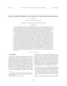
FIG. 6. Cross section of the model area from west to east through, approximately, Tabentis and Inferta, showing simulated potential temperature. The x axis indicates distance from the shoreline.

southeast coast of the island. This result is in agreement with the conclusions of Arritt (1993), who found that the maximum sea-breeze perturbation developed for weak, opposing large-scale flow. The thermally driven wind component also is strong at the foothills of the mountains at the southeastern part of the island. A likely explanation is the development of anabatic winds, which are superposed on the sea breeze. Last, at 2000 LST the land surface is only slightly warmer than the water, and the model simulations indicate that most of the sea-breeze circulations have ceased (Fig. 2d). The winds over most of the island are weak and variable. The exception is the sea-breeze system in the western part of the island, which is superposed on the northwest synoptic flow. It continues to blow, but with reduced strength and penetration. A notable feature of the simulated wind field is the appearance of a cyclonic eddy pattern south of Cagliari in the late afternoon–early evening. The eddy is about 50 km in diameter and develops as a result of the interaction between the northwesterly flow from Campidano Valley and the flow that goes around the island directing toward northeast. A similar eddy pattern was found in many previous numerical studies (e.g., Abbs 1986; McKendry 1992; Grisogono et al. 1998). A common feature of these studies is that eddy patterns form in the late afternoon during days with well-developed sea breezes. However, because of the detailed observations required, there is only limited observational evidence on the existence of similar features (e.g., Abbs 1986; McKendry and Revell 1992).

b. Vertical structure of the PBL Figure 5 shows the vertical structure of the boundary layer at 1300 LST at a grid point that corresponds approximately to the location of the rawinsonde station at Cagliari. Model results are shown with a full line with triangles, and the circles represent the average rawinsonde profiles (see section 2 for details). Before proceeding to the comparison of the results, it is worth mentioning that there are some peculiarities in the results of the numerical models. The MIUU model produces grid volume averages, the dimensions of the grid cells being different in different parts of the model domain (because of the telescoping grid). In the part of the model domain that corresponds to the location of Cagliari, the grid distance in the horizontal is about 5 km, and thus the results presented in Fig. 5 correspond to a site that is located about 5 km from the shoreline although Cagliari is a coastal city. From the simulated wind speed and direction profiles (Fig. 5), it is recognized that the depth of the sea-breeze layer is between 400 and 800 m. The wind in the sea-breeze layer is from southerly directions while, in the layer above it, northeasterly flow prevails. The return flow merges with the prevailing synoptic flow and is difficult to distinguish. Notice also the broad maximum in the sea-breeze profile at approximately 200 m AGL. The observations indicate a backing of the wind with height in opposition to the frictionally induced rotation. The numerical model simulates a similar rotation of the wind with height, with the exception of the transition layer between the sea

APRIL 2000

MELAS ET AL.

523

FIG. 7. Same as Fig. 6 but for the wind speed.

breeze and the overlying synoptic flow in which the model result deviates from the observed wind direction. This ‘‘paradoxical’’ behavior of the wind direction most likely is associated with baroclinicity. This likelihood was confirmed by performing some additional simulations for which the thermal wind was set to zero. In this case, the resulting profiles indicated a veering of the wind with height. Last, both the observed and the modeled potential temperature profiles indicate the existence of a shallow convective layer of about 400 m. Similar results were obtained by Melas et al. (1998a) and were attributed to the strong cold-air advection from the sea. Figures 6 and 7 show cross sections of the model area from west to east through, approximately, Tabentis and Inferta, showing simulated potential temperature and wind speed, respectively. As seen in Fig. 6, the boundary layer over water is characterized by stable stratification resulting from the low potential temperature of the water surface. The vertical temperature gradient in the lowest layer is, on the average, 68C (100 m)21 . As the cold air flows across the shoreline, it experiences an abrupt change in surface conditions such as roughness, temperature, and wetness and is modified extensively by the underlying surface. The adjustment of the onshore flow is accomplished gradually within a thermal internal boundary layer (TIBL) that is developing with distance downwind of the coast (Melas and Kambezidis 1992). The vertical structure of the potential temperature within the TIBL reveals strong convective effects, with intense mixing leading to a well-mixed layer that is shallow (;50 m) near the coastline but is developing rapidly to over 500 m a few kilometers from the shoreline. On the other hand, the wind speed is decreasing

gradually with distance downwind of the shoreline (Fig. 7). This decrease mainly is attributable to the higher roughness of the land surface but also indicates the blocking effect of the mountain. The same conclusions were found in Sempreviva et al. (1994a, b), in which 2 yr of data were analyzed. Notice also the elevated maximum in wind speed at about 100 m, which corresponds to the layer of maximum sea-breeze intensity. This height is appreciably lower than the corresponding height at the south coast of the island. 5. Concluding remarks A three-dimensional, higher-order closure model for complex terrain is applied to simulate the flow dynamics over the island of Sardinia during summer conditions characterized by weak synoptic forcing from the northwest sector and clear skies. These conditions favor the development of local circulations, the most important being the katabatic winds and the sea-breeze systems. In consequence, the simulated wind fields are variable both in time and space, with the following characteristics. 1) During nighttime, the winds over most parts of the island are low, and there is substantial evidence for the development of strong katabatic winds. There also are indications of the development of land breezes. The land-breeze direction is similar to that of the drainage flow, however, and it is difficult to differentiate the individual local wind components. 2) During daytime, several sea-breeze systems develop in the area where the wind has an onshore component

524

JOURNAL OF APPLIED METEOROLOGY

at virtually every coastline. The strongest thermally induced wind is simulated at the southern coast of the island, that is, for opposing synoptic flow. 3) The interaction between the different sea-breeze systems produces convergence zones accompanied by upward motion. 4) The sea breeze at the city of Cagliari is from southerly directions and occupies a layer of approximately 400 m. The wind profile exhibits a wide maximum of about 6 m s21 at about 200 m. 5) Cold air advection leads to the development of TIBLs. The depth of the mixed layer near the coastline is only a few tens of meters, gradually increasing to over 500 m a few kilometers from the shoreline. Acknowledgments. The work described herein was carried out when the first author was visiting the Institute of Atmospheric Physics at CNR in Rome, Italy. This visit was within the frame of the EU programme, ‘‘Human Capital and Mobility,’’ and was supported by the EU contract ERBCHRXCT940518. The current version of the paper benefited greatly from the comments of one of the anonymous reviewers, to whom the authors are indebted. REFERENCES Abbs, D. J., 1986: Sea-breeze interactions along a concave coastline in southern Australia: Observations and numerical modeling study. Mon. Wea. Rev., 114, 831–848. Andre´n, A., 1990: Evaluation of a turbulence closure scheme suitable for air-pollution applications. J. Appl. Meteor., 29, 224–239. Arritt, R. W., 1993: Effects of the large-scale flow on characteristic features of the sea breeze. J. Appl. Meteor., 32, 116–125. Atkinson, B. W., 1981: Mesoscale Atmospheric Circulations. Academic Press, 495 pp. Deardorff, J. W., 1978: Efficient prediction of ground surface temperature and moisture, with inclusion of a layer of vegetation. J. Geophys. Res., 83, 1889–1903. Enger, L., 1984: A three-dimensional time-dependent model for the meso-g-scale—Some test results with a preliminary version. Report No. 80, Department of Meteorology, Uppsala University, Uppsala, Sweden, 25 pp. plus figs. [Available from Department of Earth Sciences, Meteorology, Villavaegen 16, 75236 Uppsala, Sweden.] , 1986: A higher-order closure model applied to dispersion in a convective PBL. Atmos. Environ., 20, 879–894. , 1990: Simulation of dispersion in moderately complex terrain. Part A. The fluid dynamic model. Atmos. Environ., 24, 2431– 2446. , and B. Grisogono, 1998: The response of bora-type flow to sea surface temperature. Quart. J. Roy. Meteor. Soc., 124, 1227– 1244.

VOLUME 39

, D. Koracin, and X. Yang, 1993: A numerical study of boundarylayer dynamics in a mountain valley. Bound.-Layer Meteor., 66, 357–394. Grisogono B., L. Stro¨m, and M. Tjernstro¨m, 1998: Small-scale variability in the coastal atmospheric boundary layer. Bound.-Layer Meteor., 88, 23–46. Ludwig, F. L., 1983: A review of coastal zone meteorological processes important to the modeling of air pollution. Proc. 14th Int. Tech. Meeting on Air Pollution Modeling and its Application, Copenhagen, Denmark, NATO Committee on Challenges of Modern Society, 225–257. McKendry, I. G., 1992: Numerical simulation of sea-breeze interactions over the Auckland region of New Zealand. N. Z. J. Geol. Geophys., 35, 9–20. , and C. G. Revell, 1992: Mesoscale eddy development over South Auckland—A case study. Wea. Forecasting, 7, 134–142. Melas, D., and H. D. Kambezidis, 1992: The depth of the internal boundary layer over an urban area under sea-breeze conditions. Bound.-Layer Meteor., 61, 227–264. , I. C. Ziomas, and C. S. Zerefos, 1995: Boundary layer dynamics in an urban coastal environment under sea breeze conditions. Atmos. Environ., 29, 3605–3617. , , O. Klemm, and C. S. Zerefos, 1998a: Anatomy of the sea-breeze circulation in the Athens area under weak large-scale ambient winds. Atmos. Environ., 32, 2223–2237. , , , and , 1998b: Flow dynamics in the Athens area under moderate large-scale winds. Atmos. Environ., 32, 2209–2222. Pielke, R. A., 1984: Mesoscale Meteorological Modeling. Academic Press, 612 pp. Sempreviva, A. M., A. Lavagnini, and D. Melas, 1994a: Experimental study of flow modification in the coastal Mediterranean area. Application of a mesoscale model. Proc. Fifth European Wind Energy Association Conf., Thessaloniki, Greece, Hellenic Wind Energy Association and European Wind Energy Association, 214–221. , , and V. Quesada, 1994b: Experimental test of the EEC wind climatology model in a Mediterranean coastal area. Nuovo Cimento, 17, 595–604. Tjernstro¨m, M., 1987: A study of flow over complex terrain using a three dimensional model. A preliminary model evaluation focusing on stratus and fog. Ann. Geophys., 5B, 469–486. , 1988: Numerical simulations of stratiform boundary layer clouds on the meso-g-scale. Part 1: The influence of terrain height differences. Bound.-Layer Meteor., 44, 33–72. Wieringa, J., 1993: Representative roughness parameters for homogeneous terrain. Bound.-Layer Meteor., 4, 323–349. Yamada, T., 1977: A numerical simulation of pollutant dispersion in a horizontally homogeneous atmospheric boundary layer. Atmos. Environ., 11, 1015–1024. , and G. L. Mellor, 1975: A simulation of the Wangara atmospheric boundary layer data. J. Atmos. Sci., 32, 2309–2329. Yang, X., 1991: A study of nonhydrostatic effects in idealized sea breeze systems. Bound.-Layer Meteor., 54, 183–208. Zhong, S., and E. S. Takle, 1993: The effects of large-scale winds on the sea-breeze circulations in an area of complex coastal heating. J. Appl. Meteor., 32, 1181–1195.