Drizzle in Stratiform Boundary Layer Clouds. Part I - AMS Journals

VOLUME 62

JOURNAL OF THE ATMOSPHERIC SCIENCES

SEPTEMBER 2005

Drizzle in Stratiform Boundary Layer Clouds. Part I: Vertical and Horizontal Structure R. WOOD Met Office, Exeter, Devon, United Kingdom (Manuscript received 2 April 2004, in final form 16 February 2005) ABSTRACT Detailed observations of stratiform boundary layer clouds on 12 days are examined with specific reference to drizzle formation processes. The clouds differ considerably in mean thickness, liquid water path (LWP), and droplet concentration. Cloud-base precipitation rates differ by a factor of 20 between cases. The lowest precipitation rate is found in the case with the highest droplet concentration even though this case had by far the highest LWP, suggesting that drizzle can be severely suppressed in polluted clouds. The vertical and horizontal structure of cloud and drizzle liquid water and bulk microphysical parameters are examined in detail. In general, the highest concentration of r ⬎ 20 ␮m drizzle drops is found toward the top of the cloud, and the mean volume radius of the drizzle drops increases monotonically from cloud top to base. The resulting precipitation rates are largest at the cloud base but decrease markedly only in the upper third of the cloud. Below cloud, precipitation rates decrease markedly with distance below base due to evaporation, and are broadly consistent in most cases with the results from a simple sedimentation– evaporation model. Evidence is presented that suggests evaporating drizzle is cooling regions of the subcloud layer, which could result in dynamical feedbacks. A composite power spectrum of the horizontal spatial series of precipitation rate is found to exhibit a power-law scaling from the smallest observable scales to close to the maximum observable scale (⬃30 km). The exponent is considerably lower (1.1–1.2) than corresponding exponents for LWP variability obtained in other studies (⬃1.5–2), demonstrating that there is relatively more variability of drizzle on small scales. Singular measures analysis shows that drizzle fields are much more intermittent than the cloud liquid water content fields, consistent with a drizzle production process that depends strongly upon liquid water content. The adiabaticity of the clouds, which can be modeled as a simple balance between drizzle loss and turbulent replenishment, is found to decrease if the time scale for drizzle loss is shorter than roughly 5–10 eddy turnover time scales. Finally, the data are compared with three simple scalings derived from recent observations of drizzle in subtropical stratocumulus clouds.

1. Introduction Drizzle is an important phenomenon in marine low cloud because (i) even low precipitation rates are comparable energetically to other forcings, and (ii) drizzle is common in the marine boundary layer (MBL) (Petty 1995). Drizzle production is dependent upon the interplay between microphysical, thermodynamic, and dynamical processes (Mason 1952; Nicholls 1987; Baker 1993; Austin et al. 1995b; Feingold et al. 1996). The hypothesis (Liou and Ou 1989; Albrecht 1989) that enhanced aerosol concentrations in MBL clouds may suppress drizzle and prolong cloud lifetime (the so-called

Corresponding author address: Dr. Robert Wood, Dept. of Atmospheric Sciences, University of Washington, Box 351640, Seattle, WA 98102. E-mail: [email protected]

second indirect effect, or aerosol–cloud lifetime effect) has generated a need to quantify the magnitude of this effect. So far, however, there exists little direct evidence to support or deny the initial hypothesis. This is hardly surprising given the complexity of the processes involved and our inability to isolate aerosol effects from changes in meteorology. To simplify the hypothesis, it may be useful to split it conceptually into three separate process hypotheses, each of which must be verified: • H1: Changes in aerosol concentrations result in

changes to the cloud droplet size distribution (DSD), all other controlling variables being held constant. The simplest change that may occur is that increased aerosol concentrations lead to increased concentrations of cloud droplets and therefore smaller droplets. • H2: The aerosol-induced changes to the cloud DSD

3011

JAS3529

3012


VOLUME 62

result in changes in the collision–coalescence rates that in turn lead to changes in the precipitation rate. The simplest form of this is that smaller, more numerous cloud droplets suppress coalescence rates, for a fixed liquid water content. • H3: Changes in precipitation rate result in changes in the distribution and/or total amount of liquid water that in turn affects the radiative properties of the cloud. Verification of H1, H2, and H3 is necessary, but not sufficient to determine the climatological significance of the second indirect effect: placing the hypotheses into a quantitative, global framework is likely to remain a challenge for some time. Evidence supporting H1 first emerged in the 1950s (e.g., Lewis 1951; Twomey 1959; Twomey and Warner 1967). A wealth of subsequent observations (Martin et al. 1994; Gultepe et al. 1996; Brenguier et al. 2000; Durkee et al. 2000; Ackerman et al. 2000; Taylor et al. 2000; Brenguier 2003) have confirmed H1, although the climatological significance remains uncertain (Haywood and Boucher 2000), and the relationship between aerosol and cloud droplet number concentration is complex (Gultepe et al. 1996; Snider et al. 2003). Differing aerosol size distributions and chemical compositions (Pruppacher and Klett 1997), updraft speeds (Snider et al. 2003), entrainment (Korolev and Isaac 2000), radiative growth (Austin et al. 1995a; Harrington et al. 2000), and ripening effects (Celik and Marwitz 1999; Wood et al. 2002) all complicate this relationship and need to be better quantified, particularly on the large-scale using satellites (Nakajima et al. 2001; Breon et al. 2002; Schuller et al. 2003). There is less evidence for H2, probably because drizzle has traditionally been considered a secondary property of MBL clouds and has not been the primary focus of observational studies. Yum et al. (1998) and Yum and Hudson (2002) show decreasing drizzle liquid water contents in stratus as cloud droplet concentration Nd increases. Hudson and Yum (2001) find this to be the case in small cumuli, and Comstock et al. (2004) find a significant negative correlation between drizzle rate and Nd in southeast Pacific stratocumulus. Recent observational studies of subtropical marine stratocumulus by Pawlowska and Brenguier (2003) and vanZanten et al. (2005) find that the precipitation rate at cloud base is inversely proportional to droplet concentration for fixed cloud thickness, providing further evidence for H2. The current status of evidence for H2 is summarized in Fig. 1, which shows precipitation rate [R(zCB), nominally at the cloud base] versus Nd for MBL clouds from around the world. Despite considerable spread in the

FIG. 1. Precipitation rate [R(zCB), at cloud base unless specified otherwise] as a function of the cloud droplet concentration Nd in boundary layer clouds. The data are collated using a number of field programs around the world, using mainly in situ aircraft data, but also include recent remote sensing observations. Those measurements for which LWP data are available are shaded, with high LWP being darker. The published data are taken from ASTEX Lagrangian 1 (Bretherton and Pincus 1995), Dynamics and Chemistry of Marine Stratocumulus (DYCOMS-II; vanZanten et al. 2002), North Sea stratocumulus (Nicholls and Leighton 1986), EPIC (Bretherton et al. 2004), averages from a number of field campaigns (Yum et al. 1998), and northeast Atlantic flights (Pawlowska and Brenguier 2003). The Yum and Hudson (2002) measurements were presented as cloud mean drizzle liquid water content qD rather than precipitation rate and converted to precipitation rate using the transformation R ⫽ 38q1.08 D , the best fit relation (r ⫽ 0.90) derived from the microphysical observations of 12 flights in this study. The (Pawlowska and Brenguier 2003) values are mean precipitation rates over the entire cloud layer in each case. The correlation coefficient between ln Nd and ln R(zCB) is r ⫽ ⫺0.6, significant at the 99% level.

precipitation rates for any given Nd, there is a distinct trend with reduced precipitation rate as the cloud droplet concentration increases. Evidence for H2 on the regional to global scale is lacking at present because current satellite radar observations are not sensitive enough to detect the weak returns associated with MBL drizzle. This situation will change, however, with the launch of the Cloudsat mission (Stephens et al. 2002). Observations of radar reflectivity returns from MBL clouds need to be converted to physically significant drizzle parameters (i.e., precipitation rate) before they are useful (Comstock et al. 2004; vanZanten et al. 2005). Such relations will be examined in Wood (2005, hereafter Part II). An absence of control conditions precludes purely observational evidence for H3. Changes to the radiative properties of the cloud implied in H3 can include

SEPTEMBER 2005

WOOD

changes in the vertically integrated liquid water path, changes in the cloud fractional coverage, or a mixture of both. There is some evidence suggesting that the degree of adiabaticity of MBL clouds is reduced when the precipitation rate becomes high (Gerber 1996; see also this study). However, it may be that the presence of drizzle could lead to less adiabatic, but deeper, clouds with the same liquid water path (LWP), so the radiative effects of precipitation are difficult to assess. The hypothesis H3 is more amenable to study with high-resolution large eddy simulations (LES; Feingold et al. 1997; Khairoutdinov and Kogan 1999; Stevens et al. 1998). Of these studies, Feingold et al. (1997) and Stevens et al. (1998) demonstrate that, in the presence of heavy drizzle, cloud layers have lower integrated water contents, directly supportive of H3. There is also no shortage of GCM simulations that demonstrate H3 (see review of Haywood and Boucher 2000). However, these simulations necessarily depend upon very simple bulk parameterizations of drizzle production that are poorly constrained. In Part II of this study, we compare bulk microphysical parameterizations with rates estimated by application of the stochastic collection equation to observed drop size distributions. It is now widely acknowledged that considerable spatial variability of cloud LWP is the rule rather than the exception (Cahalan et al. 1994; Szczodrak et al. 2001; Wood and Taylor 2001; Wood and Hartmann 2005a, manuscript submitted to J. Climate). It is perhaps not surprising; therefore, that recent work has shown that drizzle in stratocumulus clouds tends to occur in intermittent localized patches (Austin et al. 1995b; Vali et al. 1998; Stevens et al. 2003; Comstock et al. 2004, 2005; vanZanten et al. 2005) rather than being uniformly spread through the cloud. The patches have a wide variety of scales (Vali et al. 1998) and, on the mesoscale (scales of a few kilometers or more), tend to occur in regions where the cloud thickness is locally enhanced (K. Comstock 2004, personal communication). At smaller scales it is uncertain how cloud thickness variations affect drizzle production, and eddy dynamics may become important. Thicker regions of cloud contain larger cloud droplets and higher liquid water contents near cloud top than thinner regions, and the relationship between cloud liquid water content and coalescence rate is strongly nonlinear (Nicholls 1987; Austin et al. 1995b). Evidence has been presented (Paluch and Lenschow 1991; Rand 1995; Jensen et al. 2000; Comstock et al. 2005) suggesting that the evaporative cooling of drizzle below cloud base may drive mesoscale circulations that affect the thermodynamic and cloud evolution in the MBL (Stevens et al. 1998). We exam-

3013

ine the potential coupling between cloud liquid water variability and drizzle variability in this study. The study comprises two parts. In Part I, aircraft observations of the horizontal and vertical structure and variability of cloud and drizzle are described in 12 stratiform boundary layer cloud cases over the northeast Atlantic and in U.K. coastal waters. The clouds examined have a considerable variety of droplet concentrations, LWP, and drizzle rates, which allows us to make inferences about (i) the role of droplet concentration and LWP upon the production of drizzle and (ii) the effects of drizzle upon the adiabaticity of liquid water content. Aerosol microphysics (i.e., H1) is not considered explicitly in this study. Part II of the study presents a more detailed analysis of the size resolved microphysics and the related issues of radar reflectivity–precipitation rate relationships and the parameterization of warm cloud microphysical processes. Section 2 presents details of the flights and instrumentation. Section 3 examines the vertical structure of the cloud and drizzle parameters. Section 4 describes mesoscale horizontal variability of the drizzle, its scaling and intermittency, and section 5 examines the time scales involved in drizzle processes. There is discussion and an attempt to generalize the findings here, before concluding with suggestions for future work.

2. Case details a. Flights Data in this study were collected using the Met Office C-130 aircraft. Twelve flights are presented with eleven during the day over U.K. oceanic waters and one (A209) at night as part of the Atlantic Stratocumulus Transition Experiment (ASTEX) first Lagrangian experiment in the northeast Atlantic Ocean (Bretherton and Pincus 1995). The sampling strategy differed between flights, although in each case there is good sampling of the vertical and horizontal structure of the cloud. In all flights the mean aircraft position followed an approximately Lagrangian path, drifting with the mean wind in the MBL. Flights consisted of a series of straight and level runs in, above, and below cloud together with a number of vertical ascents from above cloud to close to the surface (⬃15 m). Most flights were augmented with a series of “porpoise” runs up and down through the cloud to improve vertical sampling. Where possible, a run close to the surface (⬃30 m) characterized lower boundary conditions. Straight and level runs were typically 60 km in length, but flights A648 and A649 comprised a greater number of shorter runs (20 km).

3014


VOLUME 62

TABLE 1. Flight numbers, dates, locations, times, cloud type, mean heights of cloud base zCB and cloud top zi, mean liquid water path LWP (⫾ error), mean in-cloud droplet concentration N*, and mean cloud-base precipitation rate RCB. Note that the errors are errors in the mean value and not estimates of the variability in that parameter.

Flight A049 A209 A439 A641 A644 A648 A649 A693 A762 A763 A764 A767

Date 6 12 29 3 14 28 29 8 12 14 15 28

Dec 90 Jun 92 Feb 96 Dec 98 Dec 98 Jan 99 Jan 99 Jul 99 Jun 00 Jun 00 Jun 00 Jun 00

Location

Local time (h)

Type

zCB (m)

zi (m)

LWP (g m⫺2)

N* (cm⫺3)

RCB (mm day⫺1)

SW of U.K. Azores NW Ireland North Sea SW of UK SW of U.K. SW of U.K. NW Ireland SW of U.K. SW of U.K. SW of U.K. North Sea

12–15 00–04 12–15 11–16 12–15 12–15 12–16 12–16 12–16 12–16 12–16 12–15

Sc Sc Sc Sc St St Sc St/Sc St/Sc St/Sc St/Sc Sc w/Cu

825 ⫾ 23 310 ⫾ 44 780 ⫾ 19 430 ⫾ 7 150 ⫾ 75 190 ⫾ 18 450 ⫾ 9 115 ⫾ 21 180 ⫾ 13 245 ⫾ 18 ⬇20** 935 ⫾ 24

1450 ⫾ 34 705 ⫾ 27 1150 ⫾ 9 1110 ⫾ 14 1800* 1550* 775 ⫾ 13 395 ⫾ 3 495 ⫾ 11 485 ⫾ 14 320 ⫾ 6 1350 ⫾ 10

260 ⫾ 44 170 ⫾ 34 100 ⫾ 15 360 ⫾ 16 90 ⫾ 50 85 ⫾ 50 80 ⫾ 6 80 ⫾ 3 80 ⫾ 5 45 ⫾ 2 70 ⫾ 6 90 ⫾ 10

310 120 90 420 20 8 60 110 95 85 65 110

0.49 0.47 0.24 0.054 0.66 1.12 0.095 0.41 0.28 0.34 0.44 0.78

* The cloud consisted of two or more layers that were heterogeneous and often had indistinct vertical boundaries. The figure for mean cloud top given is for the uppermost layer. ** The aircraft was not able to descend to cloud base because of visibility restrictions. This cloud base was estimated by extrapolation of the profiles of liquid water content from higher levels.

b. Instrumentation and data analysis methods The dynamic and thermodynamic measurement system and associated errors are described in more detail in Rogers et al. (1995). Cloud microphysical measurements were made at 1 Hz using a Particle Measuring Systems, Inc. (PMS) Forward Scattering Spectrometer Probe (FSSP) (Baumgardner et al. 1993) that counts and sizes particles into 15 size bins in the radius range 1–23.5 ␮m. Larger particles were measured using a PMS 2D-C optical array probe that counts and sizes particles into 32 size bins in the radius range 12.5–400 ␮m. For the 2D-C data the first size bin is not used as there is large uncertainty in the sizing of particles in this bin (Korolev et al. 1998). Combined FSSP and 2D-C size distributions are produced by linear interpolation in log(dN/dr)–logr coordinates. Further details of the size resolved microphysics, including sampling issues and the parameters derived therefrom, are presented in Part II. Turbulent variance and covariance flux measurements were derived from horizontal runs by first detrending the time series using a 3-km-wide moving triangular filter and then using eddy correlation. Sea surface temperature (SST) is estimated from a run at the lowest flight level using a Heinmann PRT4 radiometer. Ten-meter wind speed U10 is estimated using the mean wind speed at the lowest flight level and extrapolating this measurement down using a logarithmic wind profile (Bretherton and Pincus 1995) using a roughness length of 5 ⫻ 10⫺4 m. Friction velocity u is * estimated using momentum fluxes from the lowest flight leg. Convective velocity scale w is estimated us*

ing the buoyancy integral method (Nicholls and Leighton 1986). In some cases the buoyancy integral is negative due to low buoyancy generation in cloud or because the air was being cooled by a lower SST, and in these cases w cannot be defined. *

c. Case details and overviews Table 1 gives details of the dates and locations, together with some mean properties of the clouds measured. Cases are referred to by flight number throughout. There is a considerable range of mean LWP (45– 360 g m⫺2), droplet concentration (8–420 cm⫺3), and cloud-base precipitation rate (0.054–1.12 mm day⫺1) between flights. Liquid water path is estimated by vertical integration of liquid water content using a number of ascents/descents through the cloud layer. We calculate the mean droplet concentration using all samples in the height range 1/3 ⬍ z ⬍ 2/3 to avoid sampling re* gions close to cloud base and cloud top, where z is a * normalized height given by z ⫺ zCB , z ⫽ * zi ⫺ zCB

共1兲

where zCB and zi are the mean cloud-base height and cloud top, respectively, and z is the height of a particular measurement. Because it is not possible to assign a local cloud base to every measurement, it is possible, due to the spatial and temporal variability in the cloud geometrical properties, that a measurement at height z could be either above or below cloud base when z ⫽ 0. *

SEPTEMBER 2005

3015

WOOD

TABLE 2. Thermodynamic and dynamic details of the cases studied. From left to right: sea surface temperature (SST); 10-m wind speed U10; friction velocity u*; mean in-cloud value of the vertical wind speed standard deviation ␴w; mean in-cloud vertical wind integral scale ␭w; ratio of inversion height to the Monin–Obukhov length ⫺zi/LMO; mean inversion jump in virtual potential temperature ⌬␪␷; and mean inversion jump in total water content ⌬qT. Case

SST (K)

U10 (m s⫺1)

u* (m s⫺1)

w* (m s⫺1)

␴w (m s⫺1)

␭w (m)

⫺zi/LMO (m)

⌬␪␷ (K)

⌬qT (g kg⫺1)

A049 A209 A439 A641 A644 A648 A649 A693 A762 A763 A764 A767

283.3 290.3 281.6 282.5 284.7 283.9 283.6 286.4 286.5 287.2 287.7 285.1

5.1 8.1 6.2 0.7 9.7 13.3 2.2 10.7 11.3 7.3 1.3 10.1

0.19 0.26 0.25 0.13 0.47 0.37 0.14 0.34 0.40 0.18 0.14 0.38

0.63 0.66 0.89 0.97 — 0.33 0.62 0.43 — — 0.44 0.95

0.58 0.70 0.59 0.65 0.37 0.25 0.28 0.38 0.30 0.26 0.28 0.50

175 150 130 230 200 200 180 35 60 160 80 130

14.6 40.9 18.0 166 ⫺0.50 0.28 34.8 0.81 ⫺0.27 ⫺0.84 12.4 6.25

5.7 2.9 5.5 4.3 n/a* n/a* 2.7 5.4 4.4 4.8 2.3 3.6

⫺2.0 ⫺1.0 ⫺3.6 ⫺0.5 n/a* n/a* ⫺1.1 ⫺0.8 ⫺0.9 ⫺0.3 ⫺0.5 ⫺2.7

* These cases contained multiple weak inversions (⌬␪␷ ⬍ 1 K; ⌬qT ⬍ 0.5 g kg⫺1) both in and above the cloud layers and it is therefore not possible to define a good measure of the inversion jumps.

We calculate the cloud-base precipitation rate RCB as being the average precipitation rate for 0 ⬍ z ⬍ 1/3. * Dynamic and thermodynamic parameters are given in Table 2. Turbulent kinetic energy (TKE) in the MBL is generated by buoyant generation, shear generation, or a mixture of the two. In boundary layers driven predominantly by shear generation the vertical wind variance scales well with u (see, e.g., Nicholls and Leigh* ton 1986), and we find this for cases A644, A648, and A762. A measure of the relative roles of shear and surface buoyancy production of TKE is given by the ratio of the boundary layer depth zi to the Monin– Obukhov length LMO. Large positive values of ⫺zi/ LMO indicate that turbulence is driven primarily by thermal convection. Small negative values indicate that shear generation of turbulence dominates. Our definition of LMO accounts for the fact that cloud-top cooling in addition to surface forcing can be an important source of buoyancy generation, so we use the definition LMO ⫽ ⫺ziu3 /kw3 (see, e.g., Stull 1988), where k ⫽ 0.4 * * is the von Kármán constant. Table 2 shows that flights A049, A209, A439, A641, A649, A764, and A767 are all dominated by buoyancy generation, with the other flights being driven primarily by shear. Mean in-cloud vertical wind standard deviation ␴w tends to be larger in the convectively driven cases. To assess the role of radiation in generating cloud turbulence, we simulate radiative transfer through the clouds using a four-stream radiative code (Edwards and Slingo 1996). In each case, it is assumed that no clouds are present above the boundary layer. Visual inspection of the sky during above-cloud runs indicated a very limited coverage (1 okta or less) of higher clouds in two

cases, and no clouds in the other cases. Comparisons between the observed and modeled downwelling longwave flux just above cloud confirmed that high clouds have little appreciable effect upon the radiation fields. Radiative transfer calculations indicate that longwave flux divergences ⌬LW across the boundary layer are all negative (net loss) and range from around ⫺50 W m⫺2 in cases with relative cold cloud tops and moist lower tropospheres, to ⫺85 W m⫺2 in summer cases with low moisture above the boundary layer. Shortwave flux divergences ⌬SW depend strongly upon solar zenith angle. Because all of the flights were flown at approximately the same local time each day (apart from A209 which was at night), this results in a strong winter–summer difference in ⌬SW, with relatively little absorption for the winter cases (maximum 21 W m⫺2) to magnitudes comparable to, or even greater than, ⌬LW for summer cases. For all winter cases this results in a net radiative energy loss of 30–45 W m⫺2. The net gain/ loss in the daytime summer cases is much smaller (net losses from ⫺7 to 24 W m⫺2). Only two cases had cloud layers that were clearly decoupled from the surface mixed layer (A649 and A767). The reasons for decoupling in A649 (with a mixed layer base at z ⬃ 200 m) are difficult to determine, but in A767 a high surface latent heat flux (110 W m⫺2) was promoting a warming–deepening form of decoupling (Bretherton and Wyant 1997) as the air mass had moved southward from the Arctic over the previous two days. Cumulus clouds were observed to form at the top of the surface mixed layer (⬃600 m) and in places penetrated the overlying stratocumulus layer. The other summer case boundary layers remained coupled.

3016


VOLUME 62

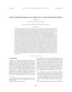
FIG. 2. Profiles of (a) temperature; (b) total water content; (c) liquid water content (line) and cloud fraction (circles); and (d) droplet concentration for flight A644. (a)–(c) Circles represent run means from 60-km horizontal runs.

The clouds and MBL observed in cases A644 and A648 were markedly different in nature to the other cases (which will be referred to throughout as well mixed). Both cases were formed in moist air masses moving northeastward from the Azores region over colder seas. Figure 2 shows profiles for A644. Surface heat fluxes in these cases were negative and a shallow (200 m deep) shear-driven mixed layer was present. Above this layer the temperature exhibited a stable lapse rate (2–3 K km⫺1) up to around 800–1000 m. Patchy layers of cloud were present at most levels in this layer. Above this layer the temperature profiles indicate a moist adiabatic lapse rate that contained less cloud than the stable layer below. This layer was capped with a weak inversion (1–3 K) at 1800–2000 m

(A644) and 1400–1600 m (A648) with layer cloud beneath. Back trajectories suggest that lower tropospheric air underwent large-scale ascent in the 24-h period prior to the observations taken on flights A644 and A648. This ascent was associated with warm frontal zones that, although the surface fronts were analyzed as being at least 100–200 km from the observational areas, appeared to have a marked effect upon the boundary layer. The ascent rates for the 24-h period prior to the observations were estimated as 0.9 and 0.8 cm s⫺1 for A644 and A648, respectively, although the trajectories suggested no large-scale ascent on A644 during the observational period, and subsidence during the observational period on A648. The mean in-cloud vertical wind integral scale ␭w is

SEPTEMBER 2005

WOOD

3017

FIG. 3. (a) Liquid potential temperature and (b) total water content in-cloud profiles for each of the cases. Layer means are subtracted in each case. The same line styles and symbols are used throughout this article whenever data from multiple flights are plotted on the same axes. Approximate measurement error is indicated on each panel.

calculated using the autocorrelation method of Lenschow and Stankov (1986). This is a measure of the horizontal distance over which the vertical wind decorrelates so that large values indicate that large coherent eddies are dominant. Typically, in a convective boundary layer this integral scale tends to be smallest at the surface increasing with height. We find this to be the case here. The integral scale tends to be smallest in clouds capping shallow boundary layers (A693, A763, and A764 all have cloud tops lower than 500 m and ␭w ⬍ 100 m) especially in those with shear-driven mixing.

3. Vertical structure a. Temperature and total water content Figure 3 shows profiles of liquid potential temperature ␪L and total water content qT in the cloud layer, referenced to the cloud layer means ␪L and q⌻ . Liq* * uid potential temperature and total water content in all cases except A644 and A648 are almost constant with height, as one would expect for a well-mixed cloud layer where the entrainment rate is small (we/w « 1). * The Rosemount E102AL total temperature sensor used

on the C-130 measures air temperature with an error of approximately 0.2–0.5 K, which is too large to determine significant deviations from adiabaticity in the well-mixed cases except close to cloud top. The deviations in A644 and A648 are significant and highlight the considerable subadiabaticity and poor vertical mixing in these cases.

b. Liquid water content and droplet concentration To facilitate the comparison between flights, N * (Table 1) is defined as the mean in-cloud droplet concentration for each case, with a 1-Hz sample defined as cloudy if the FSSP droplet concentration exceeds 5 cm⫺3 (Wood and Field 2000). Because the droplet concentrations in A644 and A648 were in places very low (⬍10 cm⫺3) we use the 1-Hz Johnson–Williams (JW) liquid water content with a threshold of 0.02 g kg⫺1 in these cases. We then calculate layer averages over a number of height bins in the range 0 ⬍ z ⬍ 1. Figure * 4 shows profiles of droplet concentration and cloud liquid water content characteristics for each flight. Cases other than A644 and A648 show similar behavior with Nd/N increasing with normalized height up to around *

3018


VOLUME 62

FIG. 4. Profiles of (a) layer mean droplet concentration Nd(z) normalized with N*; (b) standard deviation of droplet concentration at each level normalized with Nd(z); (c) adiabaticity qL(z)/qad(z); and (d) the standard deviation of the liquid water content normalized with qL(z). Symbols as for Fig. 3.

z ⫽ 0.3–0.4, then remaining approximately constant * and unity up to z ⫽ 0.8. Above this height the droplet * concentrations decrease. It is important to stress that fluctuations in cloud-base and cloud-top heights are probably the main cause of the low values close to cloud boundaries, although close to cloud base some of the droplets will be too small to be measured by the FSSP. Standard deviations of the droplet concentration at each height normalized with the mean value at that height are found to increase close to the cloud bound-

aries due to the averaging over both cloudy and clear regions. In the cloud center ␴Nd /Nd is typically 0.1–0.4 for the well-mixed cases, comparable to those presented in Noonkester (1984). In contrast, the cases A644 and A648 show larger values throughout much of the cloud layer reflecting both the broken nature and possibly the drizzle depletion of droplets in these layers. The subadiabatic nature is more easily observed using deviations of liquid water content from adiabatic

SEPTEMBER 2005

3019

WOOD

than by looking at temperature or total moisture. We define qad(z) as the adiabatic liquid water content at height z, that is, qad(z) ⫽ ⌫ad(z ⫺ zCB), where ⌫ad(T, p) is the adiabatic increase in liquid water content with height, a weak function of temperature and pressure. A single value of ⌫ad is used in each case, calculated using the mean in-cloud temperature and pressure. Then the fraction of adiabaticity is calculated as qL(z)/qad(z) for each height interval (Fig. 4c). The clouds range from close to adiabatic ( fad ⬇ 1 for A641) to highly subadiabatic with a broad range in between. Parameters that can affect the adiabaticity are drizzle loss (Stevens et al. 1998) and the balance between the transport of moisture through the cloud boundaries and the efficiency with which turbulent motions can redistribute the moisture through the layer (Wyngaard and Brost 1984; Nicholls and Leighton 1986). The normalized standard deviation of the liquid water content typically decreases through the lowest two-thirds of the cloud before increasing again as the upper boundary is reached. We define a cloud’s overall adiabaticity of the vertically integrated liquid water as fad ⫽ LWP/LWPad, where LWPad ⫽ (1/2)⌫ad(zi ⫺ zCB)2 is the adiabatic liquid water path. This measure is most accurately estimated using the vertical profiles on each flight, and the mean of the estimates for each flight is given in Table 3. The uncertainty in mean LWP due to sampling limitations is estimated using simulated profiles through a hypothetical cloud with a sinusoidal cloud base and flat top, where the local liquid water content is a constant linear function of height above the local cloud base. The amplitude of the cloud-base fluctuations is estimated using the spread in the observations of cloud-base height. Our knowledge of this amplitude is compromised by the limited sampling, but we have no means to assess this uncertainty. The horizontal wavelength is taken to be 20–40 km, typical length scales for cloud LWP fluctuations in stratocumulus clouds (Wood and Hartmann 2005b, manuscript submitted to J. Climate). The LWP and fad estimated from each sampling profile can be biased with respect to the mean for the cloud layer as a whole because of variations in cloud base. Given enough profiles for each cloud case, the hypothetical sampling model shows that the means of the LWP and fad samples yield statistically significant estimates of the cloud mean LWP and fad. A good estimate of the sampling uncertainty in mean LWP is the standard deviation of the LWP estimates from the profiles divided by the square root of the number of profiles. The standard deviation of the individual estimates is also a useful estimate of the LWP variability, but tends to underestimate the true LWP standard deviation for the hypothetical clouds by 25%–35%. The sam-

TABLE 3. Values of mean in-cloud total water content q*, cloudbase pressure pCB; temperature TCB; and ratio of observed to adiabatic LWP fad. The error in fad, given at the 1-␴ level, is estimated using a simple model of cloud structure (see text). Case A049 A209 A439 A641 A644 A648 A649 A693 A762 A763 A764 A767

q (g kg⫺1) * 5.1 10.1 4.6 3.1 8.4 6.6 6.6 9.6 9.4 9.2 8.9 4.8

pCB (hPa)

TCB (K)

928 987 940 960 996 993 972 1005 998 993 1011 909

275.5 287.3 273.9 270.7 285.1 282.0 279.7 286.0 286.0 285.7 285.0 274.6

fad 0.60 0.92 0.77 0.99 0.08 0.14 0.72 0.77 0.67 0.67 0.59 0.64

⫾ ⫾ ⫾ ⫾ ⫾ ⫾ ⫾ ⫾ ⫾ ⫾ ⫾ ⫾

0.10 0.18 0.08 0.04 0.09 0.08 0.05 0.03 0.04 0.02 0.05 0.07

pling error in fad is shown in Table 3 and does not include unknown systematic errors in the JW liquid water content sensor used to make the measurements, but these are likely to be smaller than 10% (Rogers et al. 1995). We are fairly confident about adiabaticity values in most of the clouds (see estimated errors in Table 3) and examine the possible cause of the variability among the different cases in section 5.

c. Vertical wind Vertical wind standard deviation ␴w is a signature of turbulent mixing in the cloud and ␴w (Fig. 5a) is relatively independent of height in the buoyancy-driven cases. Shear-driven cases (particularly A644 and A648) show a general decrease in ␴w with height reflecting that the turbulence is driven primarily by surface friction. The vertical wind integral scale, ␭w, varies considerably between cases, and with height in some cases (Fig. 5b). As noted in section 2c, shear-driven turbulence generally results in smaller eddies. Lenschow and Stankov (1986) find that in convective boundary layers driven by surface heating the integral scale increases with height away from the surface. Clearly it seems intuitive to find eddy sizes becoming smaller toward fixed boundaries. For turbulence generated near cloud top, as in the case of radiatively driven stratocumulus, the inversion does not impose a rigid lid to the turbulent eddies but it dampens considerably the larger eddies leading to smaller integral scales. However, gravity waves that may occur in the stable inversion layer cannot easily be distinguished from turbulent eddies in autocorrelation, and it is unclear what one should expect. Our results do not appear to show any consistent height trends in the integral scale. The integral scale is an important constraint upon simulations of the effect of

3020


VOLUME 62

FIG. 5. Profiles of vertical wind standard deviation for all cases. Symbols as in Fig. 3.

turbulence on drizzle (Austin et al. 1995b; Baker 1993) because it is related to the Lagrangian eddy time scale that, with ␴w, determines the redistribution of drizzle drops in the MBL, which controls the growth of the largest drizzle drops.

d. Drizzle bulk microphysics Drizzle drops, defined in this study as drops with radii larger than 20 ␮m, were present in all cases. We choose 20 ␮m as a separation between cloud and drizzle because it represents the approximate radius where coalescence becomes more effective than condensation (e.g., Jonas 1996). Observations of cloud DSDs (r ⬍ 20 ␮m) in warm stratiform cloud are quite common in the literature (e.g., Noonkester 1984; Nicholls 1984; Liu and Hallett 1998; Boers et al. 1996; Martin et al. 1994; Brenguier et al. 2000; Wood 2000). A much smaller number of studies exist that focus upon drizzle DSDs (e.g., Nicholls 1987; Boers et al. 1996; Wood 2000). Figure 6 shows characteristics of the populations of drizzle droplets (r ⬎ 20 ␮m) at different levels in cloud. Drizzle droplet concentrations Nd,D, liquid water contents qL,D, and precipitation rates R are all normalized with their respective in-cloud means, given in Table 4. For well-mixed cases, drizzle drop concentrations are roughly constant throughout the upper 40% of the cloud and decrease at lower levels. This demonstrates that the initial source of the drizzle drops is close to the top of the cloud where the highest liquid water contents and largest cloud droplets are. These drops may have grown to the threshold size by condensation, coalescence, or a mixture of the two; modeling results indicate

that both of these processes may be important (Nicholls 1987; Austin et al. 1995b). Drops in the radius range where both condensation and coalescence are important (⬃15–25 ␮m) are not well measured/sampled by the commonly available probes, which impedes our understanding of the sources of embryonic drizzle drops. In general, observations show that the drizzle droplet size distribution (DDSD) broadens toward clouds base. This is because drizzle drops form in the upper levels of the cloud by coalescence of cloud droplets (a process termed autoconversion). These embryonic drizzle drops then fall through cloud, growing larger by collecting cloud droplets (termed accretion) and other drizzle drops (termed self-collection). Figure 6b shows that indeed the drizzle drop size, presented here in the form of the volume radius, increases downward through the cloud. Drizzle liquid water contents (Fig. 6c) are roughly constant through the cloud and decrease only at its extremities. Precipitation rates (Fig. 6d) are roughly constant through the lowest two-thirds of the cloud and decrease above this quite markedly. This is evidence that, although most of the drizzle drops are created close to the top of the cloud through autoconversion of cloud droplets, the larger drops that dominate the precipitation rate are generated farther down in the cloud (see Part II).

e. Cloud and drizzle fraction Cloud fraction (CF) for each level is determined using the cloud droplet concentration method presented in Wood and Field (2000). The drizzle fraction is defined as the fraction of samples at each level with a

SEPTEMBER 2005

WOOD

3021

FIG. 6. Profiles of characteristics relating to the drizzle drops, which are defined here as drops with radii larger than 20 ␮m. (a) Drizzle droplet concentration Nd,D normalized with the mean drizzle droplet concentration in the cloud layer; (b) volume radius of drizzle drops r␷,D, which increases toward cloud base; (c) liquid water content contained in the drizzle drops normalized with the mean value for the cloud layer; and (d) precipitation rate normalized with the mean value in the cloud layer. Symbols are as in Fig. 3.

precipitation rate of greater than 0.5 mm day⫺1. In the well-mixed cases (Fig. 7), CF is close to unity (CF ⬎ 0.9) in the range 0.3 ⬍ z ⬍ 0.8 with a drop-off to * 0.4–0.8 at mean cloud base and top. For A644 and A648, CF ⬍ 1 at all levels. The largest CF (0.6–0.8) in these cases is found for z ⬍ 0.5, with minimum cover* age at intermediate levels, and a second peak in CF around z ⫽ 0.8–0.9. It is interesting that the frontal * cases both show considerable similarities with each pos-

sessing a two-layer cloud structure. Very low accumulation-mode aerosol concentrations (10–20 cm⫺3) were observed in the relatively clear air between the layers and above cloud in both cases, suggesting that depletion of aerosol through heavy drizzle may be rendering the upper cloud deck colloidally unstable. The lower cloud layer may have resulted from the moistening and cooling of the boundary layer caused by evaporating drizzle from the upper level. The two-layer structure

3022


VOLUME 62

TABLE 4. In-cloud mean drizzle drop concentration Nd,D, liquid water content qL,D, and precipitation rate R. Also given are cloudtop (0.8 ⬍ z ⬍ 1.0) and cloud-base (0.0 ⬍ z ⬍ 0.2) values of the * * drizzle drop volume radius r␷,D.

Case

Nd,D (L⫺1)

qL,D (10⫺3 g m⫺3)

P (mm day⫺1)

r␷, D (base) (␮m)

R␷, D (top) (␮m)

A049 A209 A439 A641 A644 A648 A649 A693 A762 A763 A764 A767

37 60 30 18 59 147 46 135 170 118 89 141

11.3 11.2 7.5 2.2 20.9 30.9 6.8 17.6 17.7 15.3 21.8 21.0

0.51 0.39 0.26 0.08 0.99 0.80 0.17 0.32 0.28 0.27 0.58 0.67

53 46 45 31 42 53 38 37 36 39 44 53

38 29 35 29 43 32 30 28 26 27 35 25

observed in both frontal cases may be a common feature of marine stratus in near-frontal warm sectors. Drizzle fraction (Fig. 7), defined using a threshold of 0.5 mm day⫺1, is substantially lower than CF at all levels for the well-mixed cases. For the two heterogeneous cases the drizzle fraction may even exceed the cloud fraction at levels between cloud layers where precipitation falling from above is present. It is interesting that the mean precipitation rate at cloud base RCB scales well with the drizzle fraction (Fig. 7 inset), suggesting that the conditional cloud-base precipitation rates for the drizzling fraction are not markedly different in each case (⬃2 mm day⫺1).

f. Moisture transport Vertical turbulent fluxes of total water content wqT are compared with the precipitation rate in Fig. 8. No flux data are available from A049 or A439. In most of the well-mixed cases there is a general balance indicating that removal of moisture by gravitational settling of drizzle drops is approximately balanced by a corresponding moisture flux, as previously observed in the ASTEX first Lagrangian case (de Roode and Duynkerke 1997). In several cases the moisture fluxes exceed the precipitation fluxes. In the two heterogeneous cases (A644 and A648), the turbulent moisture fluxes are small and in A644 actually negative throughout the cloud, indicating that drizzle in these cases is depleting cloud water. In A644 and A648, it is estimated that complete removal of the upper layers of cloud would take place in under two hours if the precipitation and turbulent moisture flux remains unchanged. This may be an example of a general transi-

FIG. 7. Profiles of (a) cloud fraction and (b) drizzle fraction for all cases. Symbols as in Fig. 3. Inset shows that the mean cloudbase precipitation rate RCB scales well with the mean drizzle fraction in the lower half of the cloud.

tion from a deep cloud-filled near-frontal layer to a more shallow MBL.

g. Subcloud microphysics Removal of cloud liquid water by drizzle and its subsequent evaporation below cloud base leads to a heat source/moisture sink in the cloud layer and a heat sink/ moisture source below it. The evaporation rate profile is therefore crucial. A simple model of the sedimentation–evaporation process is constructed to describe the evolution of a population of drizzle drops falling and evaporating below cloud base (Comstock et al. 2004). Solutions are obtained for the temperature range 270– 290 K and for the mean volume radius of drizzle drops at the cloud base r␷,D(CB) from 30 to 80 ␮m, covering the range of observations. The temperature profile below cloud base is assumed to be dry adiabatic, with a constant water vapor mixing ratio. The model results reveal that the subcloud precipitation rate profile R(z),

SEPTEMBER 2005

WOOD

3023

FIG. 8. Profiles of the vertical turbulent fluxes of total water content (filled circles) and precipitation rates for the 12 cases. Error bars on the turbulent fluxes are estimated using the integral scale method of Lenschow and Stankov (1986). Here wqT is shown positive, and R negative, for upward transport of moisture.

when normalized with the cloud-base rate RCB, depends strongly upon r␷,D(CB). A parameterization of these results (Comstock et al. 2004) fits the aircraft data reasonably well (Fig. 9) given the patchiness, and therefore limited sampling of the subcloud drizzle by the aircraft. The ability of the sedimentation–evaporation model, which is strictly valid only for a uniform DDSD, to

accurately simulate cases where cloud-base DDSD is varying horizontally, is an important issue. A strong spatial correlation between RCB and r␷,D(CB) leads to strong biases in the estimation of mean R(z) assuming a uniform DDSD because drizzle evaporation rate is strongly nonlinearly dependent upon r␷,D(CB). The biases are strongly reduced if RCB is instead better correlated with drizzle drop number concentration

3024


FIG. 9. Subcloud precipitation rates normalized with cloud-base values plotted as a function of height below cloud base normalized with the r ⬎ 20 ␮m mean volume radius of the size distribution at cloud base taken from Table 4. The dashed line is a parameterization derived from the sedimentation–evaporation model and constitutes a reasonable fit to the observations.

Nd,D(CB), and this is implied by recent observational studies (Comstock et al. 2004; vanZanten et al. 2005). However, mesoscale variability in relative humidity will also prove to be a limitation on the utility of the sedimentation–evaporation model. As a general rule, approximately 50% of the drizzle flux in the cases studied evaporates within 60 to 100 m of cloud base and 80% within 150 to 250 m of cloud base. This is likely to be a general result for drizzling stratocumulus, and is supported by observations in the southeast Pacific (Bretherton et al. 2004; Comstock et al. 2004). It is therefore more likely that drizzle feedbacks on cloud thermodynamics and structure will stem from a moistening and cooling of the subcloud layer than by a removal of moisture from the MBL except where cloud base is very low. Evaporative cooling rates (per mm day⫺1 RCB) from the model as a function of height and r␷,D(CB) (Fig. 10) can be as large as the longwave (LW) radiative cooling rate, which is generally 4–10 K day⫺1 averaged over the depth of the MBL. For RCB ⫽ 1 mm day⫺1 and r␷,D(CB) ⫽ 40 ␮m, peak subcloud cooling rates are around 12 K day⫺1 at around 100 m below cloud base. The cooling rate averaged over the 300-m-deep layer below cloud

VOLUME 62

FIG. 10. Sedimentation–evaporation model cooling rates for the evaporation of drizzle below cloud base as a function of height below cloud base and mean volume radius of the drizzle drops at cloud base. The cooling rates are expressed in K day⫺1 per mm day⫺1 of cloud-base precipitation rate. A dry adiabatic layer is assumed below cloud base. The dashed line shows the level of the peak cooling rate.

base is 7.6 K day⫺1, highlighting that even modest precipitation rates can exert relatively strong dynamical forcing on the MBL.

4. Horizontal variability Drizzle tends to occur in intermittent and localized structures, rather than being evenly distributed (Austin et al. 1995b; Stevens et al. 2003; Comstock et al. 2004, 2005). Systematic quantitative analysis of the variability has not been the focus of previous studies, and yet such variability may play a central role in drizzle processes. How is drizzle production related to the spatial variability in cloud structure? In this section we focus upon aspects of the drizzle horizontal spatial variability using a number of techniques.

a. Subcloud temperature and humidity variability Horizontal runs below cloud reveal large variability in the virtual potential temperature and specific humid-

SEPTEMBER 2005

3025

WOOD

FIG. 11. Difference between the mean subcloud virtual potential temperature (␪␷, abscissa) and mean total water (qT, ordinate) in drizzle regions and drizzle-free regions for suitable subcloud runs. The dashed line corresponds to differences caused purely by evaporation.

ity on scales larger than 1 km. Several authors have reported measurable cooling and moistening of the subcloud layer on ⬎km scales, associated with the evaporation of drizzle (Paluch and Lenschow 1991; Jensen et al. 2000; Comstock et al. 2005). Here, subcloud runs are separated into drizzling and nondrizzling regions (using a threshold R ⫽ 0.01 mm day⫺1). Time series of 10-s means are used to examine scales ⬎1 km. We calculate the mean virtual potential temperature ␪␷ and total water qT for the drizzle and drizzle-free regions. For all subcloud runs containing 20%–80% drizzle points, the ␪␷ difference between drizzle and the drizzle-free regions is plotted against the corresponding qT difference (Fig. 11). For evaporating drizzle, assuming constant background conditions between the drizzle and drizzlefree regions, cooling and moistening are coupled. Two cases (A209 and A049) show good coupling. In most other cases the difference in qT is larger than that expected for evaporation alone. Interestingly, the drizzle regions are almost universally cooler and moister than the drizzle-free regions. With relative cooling in drizzle regions being 0.1–0.4 K, this is highly suggestive of a possible evaporative dynamic feedback.

b. Stationarity A composite power spectrum of precipitation rate is derived from all the level runs in and below cloud (Fig.

FIG. 12. Composite normalized power spectrum of precipitation rate from all in-cloud and subcloud runs. The dotted lines show the 25th and 75th percentiles. The dashed line shows the best fit power law. Each contributing spectrum was first normalized with its variance and windowed using a Hanning window before compositing.

12). Although there is considerable noise in the spectral estimates, it is clear that the spectrum follows an approximate power law relation from the smallest observed scales (2 km) to several tens of kilometers. There are examples in the literature showing power law scaling in this range for liquid water content or path (e.g., Cahalan and Snider 1989; Davis et al. 1996) and cloud-base height (Wood and Taylor 2001). However, the scaling properties of precipitation in MBL clouds have been little studied. Importantly, the magnitude of the power law exponent ␤ here is much lower than those found for LWP, having a value ␤ ⫽ 1.16 ⫾ 0.1 (2␴ level). This demonstrates heightened variability in drizzle at small scales. A similar value of ␤ ⬇ 1 was found from scanning radar observations of stratocumulus drizzle over the southeast Pacific (Wood et al. 2005). Structure functions (Davis et al. 1996) are complementary to spectral analysis, and we examine the statistical properties of the increments at scale r, namely ⌬R(r; x) ⫽ R(x ⫹ r) ⫺ R(x), 0 ⱕ r ⱕ L, where L is the length of the spatial series. Over the scale-invariant range (1–20 km), we derive the function ␨(q), defined by

具|⌬R共r兲|q典 ⬀ r␨共q兲, q ⱖ 0,

共2兲

3026


VOLUME 62

TABLE 5. Multifractal parameters H1 and C1 corresponding to the degree of smoothness and the degree of intermittency, respectively, for MBL cloud and drizzle fields in this study and the wider literature. The southeast Pacific data used are described in Bretherton et al. (2004) but H1 and C1 were estimated by the author using the method described in sections 4b and 4c. Cloud Location

Source/parameter

Northeast Atlantic This study Northeast Pacific Northeast Atlantic Southeast Pacific Southeast Pacific

Aircraft/rain rate Aircraft/rain rate Aircraft/cloud LWC Aircraft/cloud LWC Radar/reflectivity Microwave radiometer/LWP

H1

0.10 0.08

0.37

0.10

c. Intermittency Singular measures (Marshak et al. 1994; Davis et al. 1994, 1996) are used to characterize intermittency in the precipitation. Again, we use long (⬎30 km) straight and level runs and pad out the data with zeros to give a series with a length equal to an integral power of two. The padding does not seriously affect the resulting intermittency measure, for which we use |⌬R共␩; x兲| , 具|⌬R共␩; x兲|典

0 ⱕ x ⬍ L ⫺ ␩,

共3兲

where ⌬R(␩; x) is the ␩-scale precipitation rate gradient field and L is the length of the series. We focus upon coarse-grained versions of the gradient field which are considered as a function of the scales r(␩ ⬍ r ⱕ L) over which we perform spatial averaging

⑀共r; x兲 ⫽

1 r

冕

x⫹r

⑀共␩; x⬘兲 dx⬘, ␩ ⱕ x ⱕ L ⫺ r.

C1

0.28 0.29

with angle brackets being an ensemble average. A measure of the stationarity in the series is provided by H(q) ⫽ ␨(q)/q. Here H1 ⫽ ␨(1) is used to characterize the stationarity in the precipitation rate. We find that H1 ⫽ 0.12 and H2 ⫽ 0.09 for the in-cloud data, consistent with the Wiener–Khinchine theorem (Monin and Yaglom 1975; Lewis et al. 2004), which gives ␤ ⫽ 2H(2) ⫹ 1. ⌻he results indicate that the precipitation rate exhibits a greater degree of stationarity than the cloud liquid water (H1 ⫽ 0.28–0.29 for cloud liquid water content fields; Marshak et al. 1997).

⑀共␩; x兲 ⫽

Drizzle

共4兲

x

We find that the measures 具⑀(r)q典 ⬀ r⫺K(q), q ⱖ 0; that is, they are described well as power laws over some range of scales r (here, from 1 to ⬃10–20 km). Finally, we define C1 ⫽ K⬘(1), which takes values between 0 and 1, as a measure of the intermittency in the field

H1

C1

Notes

0.12 0.11

0.15 0.18

0.11

0.20

In cloud Below cloud Marshak et al. (1997) Marshak et al. (1997) Data described in Bretherton et al. (2004)

R(x) (e.g., see examples and further details in Davis et al. 1994). Davis et al. (1996) analyzed the intermittency in liquid water content in stratocumulus clouds and found C1 ⬇ 0.08–0.10. For the precipitation rate in our cases we find that values of C1 are much larger than for the cloud liquid water, with median C1 values of 0.15 and 0.18 for in-cloud and below-cloud data, respectively. Further partition shows that C1 decreases upward through the cloud, with C1 in the lower half of the cloud layer being similar to that in the subcloud layer. We find that C1 is quite well parameterized as a function of ␥R ⫽ (R/␴R)2, such that C ⬀ (1/␥R)1/2.

d. Drizzle in the multifractal plane Davis et al. (1994) and Marshak et al. (1997) introduce the mean multifractal plane as a formalism to characterize what can be thought of as two orthogonal multifractal properties of geophysical fields, namely the degree of nonstationarity/smoothness and the degree of intermittency (quantified by H1 and C1, respectively). These two properties suffice to describe the fractal properties of a wide variety of geophysical fields and can shed light upon the underlying processes controlling their structure. Table 5 gives values of H1 and C1 from a number of studies. Cloud liquid water content and LWP fields tend to group together with H1, C1 pairs of (0.25–0.35, 0.07–0.12). In situ measured precipitation rate fields from this study and remotely sensed radar reflectivity from drizzling stratocumulus during the East Pacific Investigation of Climate (EPIC) (Bretherton et al. 2004; Wood et al. 2004) also group together with H1 ⬇ 0.11– 0.12 and C1 ⬇ 0.15–0.20. This demonstrates that drizzle fields tend to be rougher and more intermittent than cloud fields in boundary layer clouds. In addition, such distinct structure for cloud and drizzle is undoubtedly indicative of universal aspects of the underlying physics

SEPTEMBER 2005

WOOD

FIG. 13. (a) Relative degree of spatial variability in cloud LWP and cloud-base (0 ⬍ z ⬍ 1/3) precipitation rate denoted by the * standard deviation normalized with the mean. (b) Relative degree of spatial variability in cloud droplet concentration measured in the center of the cloud (1/3 ⬍ z ⬍ 2/3). *

of cloud and precipitation formation in boundary layer clouds in different regions.

e. Links between LWP and drizzle variability Given that cloud water is the source of the precipitation, one is compelled to ask why statistical properties of the cloud and drizzle fields are so distinct. We hypothesize that enhanced roughness and intermittency in precipitation compared with cloud water is indicative of a nonlinear relationship in the conversion rate of cloud liquid water to precipitation (see also Part II). Figure 4 shows that, in the bulk of the cloud, the relative degree of spatial variability in cloud liquid water content is generally somewhat larger than the variability in cloud droplet concentration. Figure 13 suggests that the drizzle rate variability is indeed quite well correlated with the degree of variability in cloud LWP and that droplet concentration, in general, is less variable. The more accurate autoconversion schemes (see Part II) have a greater dependence upon liquid water content than droplet concentration. It seems reasonable to posit that drizzle production is more strongly modulated on the mesoscale by liquid water path than by droplet concentration. The liquid water path fluctuations are themselves most likely tied to fluctuations in cloud thickness related to mesoscale variability in temperature and humidity so that, in general, a greater degree of mesoscale variability is associated with a greater degree of drizzle variability. Assuming, for simplicity, that the sole modulator of precipitation rate is cloud liquid water, we find that fields with intermittency and stationarity properties

3027

FIG. 14. Stationarity and intermittency parameters H1 and C1 for simulated fields y ⫽ LWP␩ as described in the text. Shaded regions show one standard deviation from 100 realizations on either side of the mean. The intermittency C1 increases while H1 decreases, as ␩ increases. For 3.5 ⬍ ␩ ⬍ 4.5 the simulated fields display stationarity and intermittency characteristic of precipitation fields in drizzling stratocumulus.

typical of precipitation rate can be obtained from fields of LWP, where y ⫽ LWP␩, with ␩ being a tunable parameter. One-dimensional LWP fields with the observed mean multifractal properties [here, set constant with H1 ⫽ 0.3 and C1 ⫽ 0.1 are constructed using a bounded cascade model (Marshak et al. 1994)]. Each value of ␩ leads to different mean multifractal properties of the simulated y field. Figure 14 shows values of H1 and C1 as a function of ␩ for the simulated fields. For 3.5 ⬍ ␩ ⬍ 4.5, the derived fields y have H1 and C1 characteristic of observed drizzle precipitation. Although this result is by no means proof of a direct link between cloud and precipitation structure, it suggests that a strongly nonlinear dependence of precipitation generation upon cloud water can account for the spatial variability characteristics of precipitation in stratiform boundary layer clouds. Such a nonlinear dependence is consistent also with microphysical results presented in Part II.

5. Drizzle time scales The time required for the complete removal of all cloud water through rainout, assuming a constant cloud-base precipitation rate RCB, is ␶driz ⫽ LWP/RCB. For the clouds studied here (see Table 1), this rainout time scale ␶driz varies from 1.8 h (A644) to 160 h (A641). Cloud liquid water is replenished through turbulent fluxes for which a time scale ␶rep is defined. We introduce a simple equilibrium model of drizzle production where the loss of cloud water path through precipitation at cloud base RCB is balanced by a turbu-

3028


VOLUME 62

FIG. 15. Mean adiabaticity fad of the clouds studied as a function of the ratio of the rainout time scale to the eddy turnover time scale ␶driz/␶w. The error bars show the estimated uncertainties in the two parameters. Also shown are the results from an equilibrium model of drizzle production plotted as a function of ␶driz/␶rep, where ␶rep is the replenishment time scale for cloud LWP (see text).

lent replenishment that relaxes the cloud LWP back to the adiabatic value LWPad with a time scale ␶rep: d共LWP兲 LWPad ⫺ LWP ⫽ ⫺ RCB dt ␶rep ⫽

LWPad ⫺ LWP LWP ⫺ . ␶rep ␶driz

共5兲

The turbulent replenishment can be conceptualized as the effect that a newly introduced, and drizzle-free parcel has on the ensemble of older drizzle-laden parcels, that is, to shift the mean liquid water content closer to adiabatic. In equilibrium d(LWP)/dt ⫽ 0, so we rearrange (5), with the definition of adiabaticity for liquid water path fad ⫽ LWP/LWPad to give fad ⫽ 共1 ⫹ ␶repⲐ␶driz兲⫺1.

共6兲

When ␶rep/␶driz « 1, drizzle processes should not have a significant effect upon cloud adiabaticity. We might expect ␶rep to scale with the large-eddy turnover time scale, here defined as ␶w ⫽ zi/␴w. Fig. 15 shows the adiabaticity fad of the clouds plotted as a function of ␶w/␶driz. When ␶w/␶driz ⬎ 0.01–0.02, the clouds have markedly subadiabatic liquid water contents. Drizzle is not the only process, however, that can affect fad. Nicholls and Leighton (1986) estimate that a value of fad ⫽ 0.8 is a reasonable estimate of the adiabaticity due

to entrainment processes. This may overestimate the effects of entrainment, however, because several of the clouds studied in Nicholls and Leighton (1986) were drizzling and some of the subadiabaticity observed may have been related to depletion by precipitation processes rather than by entrainment. In case A641 (greatest ␶driz), fad ⬇ 1, although one might expect this cloud to be entraining considerably based upon w and ⌬␪␷ * (Table 2). However, we might also expect the effects of entrainment upon cloud liquid water content in this case to be limited because the air was very moist above the boundary layer. Assuming that drizzle is a dominant cause of subadiabaticity in our clouds, we find fad ⬃ 0.5 for ␶driz in the range (0.1–0.5) ␶w (Fig. 15). This implies that in most cases the replenishment time scale is considerably longer (2–10 times) than the eddy turnover time scale. The replenishment time scale may be linked more closely with the development of the observed mesoscale drizzle cells rather than eddies with sizes comparable with zi. Certainly, our power spectral observations show that the drizzle organization is not confined to horizontal scales comparable with the boundary layer depth, and extends to scales of tens of kilometers, with mesoscale temperature variations of a few tenths of a K. The propagation speed U of a density current of depth h can be estimated from U ⫽ 公gh⌬␪/␪ (e.g.,

SEPTEMBER 2005

WOOD

Simpson 1997), with ⌬␪ being the potential temperature deficit in the advancing cold current. For ⌬␪ ⫽ 0.2–0.5 K consistent with the results in Fig. 11, and h ⫽ 300–500 m (⬃ the subcloud layer depth), this gives U ⬇ 1.5–3 m s⫺1. Observed mesoscale wind variations are comparable to this (not shown). For cells with horizontal scales of the order of 10–30 km, the time scale for a mesoscale cellular circulation is several times longer than the eddy turnover time scale, and may explain why the clouds have lower fad than might be expected if cloud liquid water is replenished on a time scale ␶w.

6. Discussion and conclusions Aircraft observations have been presented to investigate aspects of drizzling boundary layer clouds paying particular attention to vertical and horizontal variability. Normalized variables were used where possible to facilitate comparison between cases, which separate into two broad types. Ten of the cases are unbroken, quite well mixed, and display many common properties, which, briefly summarized are (i) almost constant liquid potential temperature and total water content in the cloud layer, and linear (although mainly subadiabatic) increase in liquid water content with height; (ii) near-constant cloud droplet concentration with height; (iii) minima in normalized standard deviations (␴x /x ⬇ 0.2–0.4) of droplet concentration and liquid water content in the center of the cloud, with maxima (␴x/x ⬇ 1–1.5) close to cloud boundaries; (iv) vertical velocity standard deviations are 0.25–0.75 m s⫺1 throughout the cloud layer with no major height variation; (v) relatively constant drizzle drop concentrations (r ⬎ 20 ␮m) in the upper 40% of the cloud and decreasing below this, with drizzle drop volume radius increasing downward from 25–35 ␮m near top to 40–60 ␮m at the base; (vi) drizzle liquid water contents constitute only a small fraction (⬍10%) of the total condensed water; and (vii) precipitation rate is near constant in the lowest 60% of the cloud and decreases above this height. The findings are consistent with a source of embryonic drizzle drops near cloud top, where cloud liquid water contents are largest. Precipitation rates increase markedly below this due to accretion processes. We explore in more detail the relative contributions of autoconversion and accretion in Part II. In contrast to the well-mixed cases, two of the cases are more heteroge-

3029

neous, with broken, multiple layers, and are associated with near-frontal warm sectors. In these clouds potential temperature and total water is markedly stratified, liquid water contents are highly subadiabatic, and drizzle is prevalent throughout. Cloud properties are considerably more variable in the upper layers of these clouds. We hypothesize that these clouds may be representative of the transition from a deep, near-frontal cloud layer to a shallow subsidence-dominated MBL and that precipitation and cloud condensation nuclei (CCN) removal may be important in driving this transition. Evaporation of drizzle below cloud base is broadly consistent with the results from a simple sedimentation–evaporation microphysical model, which allows a parameterization of the evaporative cooling profile to be constructed that depends only upon cloud-base precipitation rate and drizzle drop volume radius r␷,D(CB). For values of r␷,D(CB) ⬍ 50 ␮m the cooling rate has a relatively sharp peak within 100 m of cloud base, with a strong decrease below this. For larger values of r␷,D(CB) the evaporative cooling extends over a rather deeper layer and does not have the sharp peak close to the cloud base. The former could lead to a destabilization of the subcloud layer (although still an overall stabilization of this layer with regard to the entire mixed layer). The profile of evaporative cooling, rather than simply the integrated value, could be important in determining the propensity for decoupling, and should be parameterized accurately. Horizontal spatial variability is of particular importance because most relationships between cloud properties and drizzle production tend to be strongly nonlinear. Because of this, we would expect the mean drizzle rate to be dependent upon both the mean state and the spatial variability of the cloud. The spatial variability occurs on horizontal scales that are smaller than the current state of the art general circulation model and must therefore be parameterized (e.g., Cahalan et al. 1994; Oreopoulos and Davies 1998; Pincus and Klein 2000; Rotstayn 2000; Larson et al. 2001; Wood et al. 2002). In addition, the mesoscale dynamics of boundary layer systems, and particularly the role of precipitation, are poorly understood. In this study, we examine aspects of the horizontal variability. First, we show that in the subcloud layer, regions containing drizzle are generally cooler and more moist than drizzle-free regions, which is suggestive of evaporative cooling. Such mesoscale ␪␷ (up to 0.5 K) and moisture (up to 0.3 g kg⫺1) variations may drive mesoscale circulations, as suggested in the conceptual model of Rand (1995). This mesoscale anticorrelation between temperature and moisture is also seen in cross-spectral analysis in regions dominated by boundary layer cloud (Wood and

3030


Taylor 2001). The precipitation rate exhibits scale invariance, from the smallest scale (here restricted to 2 km due to sampling limitations) up to several tens of kilometers. The scaling is quite robust in the ensemble, although sampling limitations precluded a case-by-case analysis. The adiabaticity analysis suggests that replenishment of cloud liquid water occurs on time scales significantly longer than ␶w. This is additional evidence of an important role for mesoscale circulations in drizzling MBL clouds. The power spectral scaling exponent (␤ ⫽ 1.16 ⫾ 0.10) is much lower than is observed in several other cloud parameters such as liquid water content (␤ ⫽ 1.36–1.43; Davis et al. 1996), saturation deficit/excess (implied ␤ ⫽ 1.65; Wood et al. 2002), optical thickness (␤ close to 5/3; Cahalan and Snider 1989), and LWP (␤ ⫽ 1.51; Wood and Taylor 2001), indicating that precipitation rate exhibits relatively higher fluctuations on smaller scales than other cloud-related variables. This can be accounted for by a strongly nonlinear dependence of autoconversion rate upon cloud liquid water content through which small fluctuations in liquid water content are effectively amplified to produce the drizzle fluctuations. Recent aircraft observations of subtropical stratocumulus (Pawlowska and Brenguier 2003, hereafter PB) over the northeast Atlantic and nocturnal subtropical stratocumuli over the northeast Pacific vanZanten et al. (2005, hereafter VZ) find remarkably good relationships between mean cloud-base precipitation rate RCB, the cloud thickness h, and the cloud droplet concentration Nd (with RCB ⬀ h4/Nd for PB and RCB ⬀ h3/Nd for VZ). Comstock et al. (2004) also find a good scaling from surface remote sensing observations in southeast Pacific stratocumulus, with RCB ⬀ (LWP/Nd)1.75. Figure 16 summarizes recent observational results and those in this study. Rain rates in this study agree more favorably with the VZ and Comstock et al. data than with PB, but several of the cases, most notably the very heterogeneous clouds (A644, A648) and the strongly polluted case (A641) do not agree particularly well with the other studies. It is interesting to note that the PB and VZ data both show good scaling with h3/Nd, but with a constant of proportionality that differs by approximately a factor of 5. The most likely reason for this is that h3/Nd is underestimated in the PB data, through a combination of h underestimation and Nd overestimation. Schuller et al. (2003) found that retrievals of h using a visible/near-IR estimate were regularly greater than those estimated from the in situ data. A different approach to estimate h using the in situ data (Pawlowska and Brenguier 2000) yielded cloud bases that were lower than PB, but by less than 25 m. The values of Nd in PB were derived

VOLUME 62

FIG. 16. Scaling of observed cloud-base drizzle rates RCB with (a) h3/Nd and (b) (LWP/Nd)1.75, where h is cloud thickness, Nd is cloud droplet concentrations, and LWP is liquid water path. Recent observational cases from subtropical stratocumulus regions are denoted as PB, VZ, and Comstock et al. (2004; C). Only daytime data from Comstock et al. (2004) were used because simultaneous remote sensing estimates of the cloud droplet concentration were available. Symbols as for Fig. 15.

with the aim of obtaining a value that is representative of the aerosol activation process rather than the mean value over the entire cloud. This was carried out by rejecting samples that are either close to cloud base, have significant drizzle water, or are not close to adiabatic. Although PB do not state how different their estimates of Nd are from layer mean values (used in VZ and in this study), it is clear that they will be somewhat higher.

SEPTEMBER 2005

WOOD

The relatively constant thermodynamical forcings associated with the subtropical stratocumulus regions studied in Pawlowska and Brenguier (2003), Comstock et al. (2004), and vanZanten et al. (2005) may help to explain why these studies find clear relationships between cloud-base drizzle rates and cloud structural and microphysical properties, while we do not. It is interesting to note that for adiabatic clouds LWP ⬀ h2, so the Comstock et al. (2004) scaling yields RCB ⬀ h3.75, which is close to that for Pawlowska and Brenguier (2003) and vanZanten et al. (2005). This suggests the possibility that there may exist simple relationships for drizzle production in stratocumulus clouds that may be applicable around the globe. Such relationships will prove useful for developing simple models to evaluate the effects of aerosols upon boundary layer cloud structure. All the studies show that RCB decreases with increasing Nd, but the precise dependence is not particularly clear (see also Fig. 1). Constraining these relationships will require a better understanding of the measurement systems used to determine cloud and drizzle properties and will provide important insight into the processes controlling the production of drizzle in boundary layer clouds. Acknowledgments. The author wishes to thank the staff of the Meteorological Research Flight and the C-130 aircrew and groundcrew for their dedication to collecting the data presented in this study. I am grateful to colleagues in the Met Office and elsewhere for discussions that aided the research presented in this paper. I thank Jean-Louis Brenguier, Gabor Vali, and an anonymous reviewer for their insightful and constructive reviews. REFERENCES Ackerman, A. S., O. B. Toon, J. P. Taylor, D. W. Johnson, P. V. Hobbs, and R. J. Ferek, 2000: Effects of aerosols on cloud albedo: Evaluation of Twomey’s parameterization of cloud susceptibility using measurements of ship tracks. J. Atmos. Sci., 57, 2684–2695. Albrecht, B. A., 1989: Aerosols, cloud microphysics, and fractional cloudiness. Science, 245, 1227–1230. Austin, P., S. Siems, and Y. Wang, 1995a: Constraints on droplet growth in radiatively cooled stratocumulus clouds. J. Geophys. Res., 100, 14 231–14 242. ——, Y. Wang, R. Pincus, and V. Kujala, 1995b: Precipitation in stratocumulus clouds: Observations and modeling results. J. Atmos. Sci., 52, 2329–2352. Baker, M. B., 1993: Variability in concentrations of cloud condensation nuclei in the marine cloud-topped boundary layer. Tellus, 45B, 458–472. Baumgardner, D., B. Baker, and K. Weaver, 1993: A technique for measurement of cloud structure on centimeter scales. J. Atmos. Oceanic Technol., 10, 557–565.

3031

Boers, R., J. B. Jensen, P. B. Krummel, and H. Gerber, 1996: Microphysical and short-wave radiative structure of wintertime stratocumulus clouds over the Southern Ocean. Quart. J. Roy. Meteor. Soc., 122, 1307–1339. Brenguier, J. L., 2003: Introduction to special section: An experimental study of the aerosol indirect effect for validation of climate model parameterizations. J. Geophys. Res., 108, 8627, doi:10.1029/2003JD003849. ——, and Coauthors, 2000: An overview of the ACE-2 CLOUDYCOLUMN closure experiment. Tellus, 52B, 815– 827. Breon, F.-M., D. Tanre, and S. Generoso, 2002: Aerosol effect on cloud droplet size monitored from space. Science, 295, 834– 837. Bretherton, C. S., and R. Pincus, 1995: Cloudiness and marine boundary layer dynamics in the ASTEX Lagrangian experiments. Part I: Synoptic setting and vertical structure. J. Atmos. Sci., 52, 2707–2723. ——, and M. C. Wyant, 1997: Moisture transport, lowertropospheric stability, and decoupling of cloud-topped boundary layers. J. Atmos. Sci., 54, 148–167. ——, and Coauthors, 2004: The EPIC 2001 stratocumulus study. Bull. Amer. Meteor. Soc., 85, 967–977. Cahalan, R. F., and J. B. Snider, 1989: Marine stratocumulus structure. Remote Sens. Environ., 28, 95–107. ——, W. Ridgway, W. J. Wiscombe, T. L. Bell, and J. B. Snider, 1994: The albedo of fractal stratocumulus clouds. J. Atmos. Sci., 51, 2434–2455. Celik, F., and J. D. Marwitz, 1999: Droplet spectra broadening by the ripening process. Part I: Roles of curvature and salinity of cloud droplets. J. Atmos. Sci., 56, 3091–3105. Comstock, K., S. Yuter, and R. Wood, 2004: Reflectivity and rain rate in and below drizzling stratocumulus. Quart. J. Roy. Meteor. Soc., 130, 2891–2919. ——, C. S. Bretherton, and S. E. Yuter, 2005: Mesoscale variability and drizzle in southeast Pacific stratocumulus. J. Atmos. Sci., in press. Davis, A., A. Marshak, W. Wiscombe, and R. Cahahlan, 1994: Multifractal characterizations of nonstationarity and intermittency in geophysical fields. J. Geophys. Res., 99, 8055– 8072. ——, ——, ——, and ——, 1996: Scale invariance of liquid water distributions in marine stratocumulus. Part I: Spectral properties and stationarity issues. J. Atmos. Sci., 53, 1538–1558. de Roode, S. R., and P. G. Duynkerke, 1997: Observed Lagrangian transition of stratocumulus into cumulus during ASTEX: Mean state and turbulence structure. J. Atmos. Sci., 54, 2157–2173. Durkee, P. A., and Coauthors, 2000: The impact of ship-produced aerosols on the microstructure and albedo of warm marine stratocumulus clouds: A test of MAST hypotheses 1i and 1ii. J. Atmos. Sci., 57, 2554–2569. Edwards, J. M., and A. Slingo, 1996: Studies with a flexible new radiation code. I: Choosing a configuration for a large-scale model. Quart. J. Roy. Meteor. Soc., 122, 689–720. Feingold, G., B. Stevens, W. R. Cotton, and A. S. Frisch, 1996: The relationship between drop in-cloud residence time and drizzle production in numerically simulated stratocumulus clouds. J. Atmos. Sci., 53, 1108–1112. ——, R. Boers, B. Stevens, and W. R. Cotton, 1997: A modeling study of the effect of drizzle on cloud optical depth and susceptibility. J. Geophys. Res., 102, 13 527–13 534.

3032


Gerber, H., 1996: Microphysics of marine stratocumulus with two drizzle modes. J. Atmos. Sci., 53, 1649–1662. Gultepe, I., G. A. Isaac, W. R. Leaitch, and C. M. Banic, 1996: Parameterizations of marine stratus microphysics based on in situ observations: Implications for GCMs. J. Climate, 9, 345– 357. Harrington, J. Y., G. Feingold, and W. R. Cotton, 2000: Radiative impacts on the growth of a population of drops within simulated summertime Arctic stratus. J. Atmos. Sci., 57, 766–785. Haywood, J. M., and O. Boucher, 2000: Estimates of the direct and indirect radiative forcing due to tropospheric aerosols: A review. Rev. Geophys., 38, 513–543. Hudson, J. G., and S. S. Yum, 2001: Maritime–continental drizzle contrasts in small cumuli. J. Atmos. Sci., 58, 915–926. Jensen, J. B., S. Lee, P. B. Krummel, J. Katzfey, and D. Gogoasa, 2000: Precipitation in marine cumulus and stratocumulus. Part I: Thermodynamic and dynamic observations of closed cell circulations and cumulus bands. Atmos. Res., 54, 117–155. Jonas, P. R., 1996: Turbulence and cloud microphysics. Atmos. Res., 40, 283–306. Khairoutdinov, M., and Y. Kogan, 1999: A large-eddy simulation model with explicit microphysics: Validation against aircraft observations of a stratocumulus-topped boundary layer. J. Atmos. Sci., 56, 2115–2131. Korolev, A. V., and G. A. Isaac, 2000: Drop growth due to high supersaturation caused by isobaric mixing. J. Atmos. Sci., 57, 1675–1685. ——, J. W. Strapp, and G. A. Isaac, 1998: Evaluation of the accuracy of PMS optical array probes. J. Atmos. Oceanic Technol., 15, 708–720. Larson, V. E., R. Wood, P. R. Field, J.-C. Golaz, T. H. Vonder Haar, and W. R. Cotton, 2001: Systematic biases in the microphysics and thermodynamics of numerical models that ignore subgrid-scale variability. J. Atmos. Sci., 58, 1117–1128. Lenschow, D. H., and B. B. Stankov, 1986: Length scales in the convective boundary layer. J. Atmos. Sci., 43, 1190–1209. Lewis, G. M., P. H. Austin, and M. Szczodrak, 2004: Spatial statistics of marine boundary layer clouds. J. Geophys. Res., 109, D04104, doi:10.1029/2003JD003742. Lewis, W., 1951: Meteorological aspects of aircraft icing. Compendium of Meteorology, T. F. Malone, Ed., Amer. Meteor. Soc., 1197–1203. Liou, K. N., and S. C. Ou, 1989: The role of cloud microphysical processes in climate: An assessment from a one-dimensional perspective. J. Geophys. Res., 94, 8599–8607. Liu, Y., and J. Hallett, 1998: On size distributions of cloud droplets growing by condensation: A new conceptual model. J. Atmos. Sci., 55, 527–536. Marshak, A., A. Davis, R. Cahalan, and W. J. Wiscombe, 1994: Bounded cascade models as non-stationary multifractals. Phys. Rev., E49, 55–79. ——, ——, W. Wiscombe, and R. Cahalan, 1997: Scale invariance in liquid water distributions in marine stratocumulus. Part II: Multifractal properties and intermittency issues. J. Atmos. Sci., 54, 1423–1444. Martin, G. M., D. W. Johnson, and A. Spice, 1994: The measurement and parameterization of effective radius of droplets in warm stratocumulus clouds. J. Atmos. Sci., 51, 1823–1842. Mason, B. J., 1952: Production of rain and drizzle in stratiform clouds. Quart. J. Roy. Meteor. Soc., 78, 377–386. Monin, A. S., and A. M. Yaglom, 1975: Statistical Fluid Mechanics: Mathematics of Turbulence. Vol. 2. The MIT Press, 874 pp. Nakajima, T., A. Higurashi, K. Kawamoto, and J. E. Penner, 2001:

VOLUME 62

A possible correlation between satellite-derived cloud and aerosol microphysical parameters. Geophys. Res. Lett., 28, 1171–1174. Nicholls, S., 1984: The dynamics of stratocumulus: Aircraft observations and comparisons with a mixed layer model. Quart. J. Roy. Meteor. Soc., 110, 783–820. ——, 1987: A model of drizzle growth in warm, turbulent, stratiform clouds. Quart. J. Roy. Meteor. Soc., 113, 1141–1170. ——, and J. Leighton, 1986: An observational study of the structure of stratiform cloud sheets: Part I. Structure. Quart. J. Roy. Meteor. Soc., 112, 431–460. Noonkester, V. R., 1984: Droplet spectra observed in marine stratus cloud layers. J. Atmos. Sci., 41, 829–845. Oreopoulos, L., and R. Davies, 1998: Plane parallel albedo biases from satellite observations. Part I: Dependence on resolution and other factors. J. Climate, 11, 919–932. Paluch, I. R., and D. H. Lenschow, 1991: Stratiform cloud formation in the marine boundary layer. J. Atmos. Sci., 48, 2141– 2158. Pawlowska, H., and J.-L. Brenguier, 2000: Microphysical properties of stratocumulus clouds during ACE-2. Tellus, 52B, 867– 886. ——, and ——, 2003: An observational study of drizzle formation in stratocumulus clouds for general circulation model (GCM) parameterizations. J. Geophys. Res., 108, 8630, doi:10.1029/ 2002JD002679. Petty, G. W., 1995: Frequencies and characteristics of global oceanic precipitation from shipboard present-weather reports. Bull. Amer. Meteor. Soc., 76, 1593–1616. Pincus, R., and S. A. Klein, 2000: Unresolved spatial variability and microphysical process rates in large scale models. J. Geophys. Res., 105, 27 059–27 066. Pruppacher, H. R., and J. D. Klett, 1997: Microphysics of Clouds and Precipitation. Kluwer Academic, 976 pp. Rand, H. A., 1995: Mesoscale dynamics of the marine atmospheric boundary layer. Ph.D. thesis, University of Washington, 136 pp. Rogers, D. P., D. W. Johnson, and C. A. Friehe, 1995: The stable internal boundary layer over a coastal sea. Part I: Airborne measurements of the mean and turbulence structure. J. Atmos. Sci., 52, 684–696. Rotstayn, L. D., 2000: On the “tuning” of autoconversion parameterizations in climate models. J. Geophys. Res., 105, 15 495– 15 507. Schuller, L., J.-L. Brenguier, and H. Pawlowska, 2003: Retrieval of microphysical, geometrical, and radiative properties of marine stratocumulus from remote sensing. J. Geophys. Res., 108, 8631, doi:10.1029/2002JD002680. Simpson, J. E., 1997: Gravity Currents in the Environment and the Laboratory. 2d ed. Cambridge University Press, 244 pp. Snider, J. R., S. Guibert, J.-L. Brenguier, and J.-P. Putaud, 2003: Aerosol activation in marine stratocumulus clouds: 2. Köhler and parcel theory closure studies. J. Geophys. Res., 108, 8629, doi:10.1029/2002JD002692. Stephens, G. L., and Coauthors, 2002: The CloudSat mission and the A-Train: A new dimension of space-based observations of clouds and precipitation. Bull. Amer. Meteor. Soc., 83, 1771–1790. Stevens, B., W. R. Cotton, G. Feingold, and C.-H. Moeng, 1998: Large-eddy simulations of strongly precipitating, shallow, stratocumulus-topped boundary layers. J. Atmos. Sci., 55, 3616–3638.

SEPTEMBER 2005

WOOD

——, and Coauthors, 2003: Dynamics and Chemistry of Marine Stratocumulus—DYCOMS-II. Bull. Amer. Meteor. Soc., 84, 579–593. Stull, R. B., 1988: An Introduction to Boundary Layer Meteorology. Kluwer Academic, 666 pp. Szczodrak, M., P. H. Austin, and P. B. Krummel, 2001: Variability of optical depth and effective radius in marine stratocumulus clouds. J. Atmos. Sci., 58, 2912–2926. Taylor, J. P., M. D. Glew, J. A. Coakley Jr., W. R. Tahnk, S. Platnick, P. V. Hobbs, and R. J. Ferek, 2000: Effects of aerosols on the radiative properties of clouds. J. Atmos. Sci., 57, 2656– 2670. Twomey, S., 1959: The nuclei of natural cloud formation. II. The supersaturation in clouds and the variation in cloud droplet concentration. Geofis. Pura Appl., 43, 243–249. ——, and J. Warner, 1967: Comparison of measurements of cloud droplets and cloud nuclei. J. Atmos. Sci., 24, 702–703. Vali, G., R. D. Kelly, J. French, S. Haimov, D. Leon, A. McIntosh, and R. E. Pazmany, 1998: Finescale structure and microphysics of coastal stratus. J. Atmos. Sci., 55, 3540–3564. vanZanten, M., B. Stevens, G. Vali, and D. Lenschow, 2002: The total water budget of nocturnal stratocumulus. Preprints, 15th Symp. on Boundary Layers and Turbulence, Wageningen, Netherlands, Amer. Meteor. Soc., CD-ROM, 4.7. ——, ——, ——, and ——, 2005: Observations of drizzle in nocturnal marine stratocumulus. J. Atmos. Sci., 62, 88–106. Wood, R., 2000: Parametrization of the effect of drizzle upon the

3033

droplet effective radius in stratocumulus clouds. Quart. J. Roy. Meteor. Soc., 126, 3309–3324. ——, 2005: Drizzle in stratiform boundary layer clouds. Part II: Microphysical aspects. J. Atmos. Sci., 62, 3034–3050. ——, and P. R. Field, 2000: Relationships between total water, condensed water, and cloud fraction in stratiform clouds examined using aircraft data. J. Atmos. Sci., 57, 1888–1905. ——, and J. P. Taylor, 2001: Liquid water path variability in unbroken marine stratocumulus. Quart. J. Roy. Meteor. Soc., 127, 2635–2662. ——, P. R. Field, and W. R. Cotton, 2002: Autoconversion rate bias in boundary layer cloud parameterizations. Atmos. Res., 65, 109–128. ——, K. Comstock, P. Caldwell, C. S. Bretherton, and S. E. Yuter, 2004: Drizzle and cloud structure in SE Pacific stratocumulus. Proc. 14th ICCP Int. Conf. on Clouds and Precipitation, Bologna, Italy, International Commission on Clouds and Precipitation, CD-ROM, 180. Wyngaard, J. C., and R. A. Brost, 1984: Top-down and bottom-up diffusion of a scalar in the convective boundary layer. J. Atmos. Sci., 41, 102–112. Yum, S. S., and J. G. Hudson, 2002: Maritime/continental microphysical contrasts in stratus. Tellus, 54B, 61–73. ——, ——, and Y. Xie, 1998: Cloud condensation nuclei and drizzle. Preprints, Conf. on Cloud Physics, Everett, WA, Amer. Meteor. Soc., 267–270.