[29] __ ,"A hierarchical view of decision support system software," in Proc. 16th Hawaii Int. Conf. System Sciences, Honolulu, HA,. Jan. 1983, vol. 1, pp. 482-489.
IEEE TRANSACTIONS ON SYSTEMS, MAN, AND CYBERNETICS, VOL. SMC-14, NO.5, SEPTEMBER/OCTOBER
[24] R. H. Sprague and E. D. Carlson, Building Effective Decision Support Systems. New Jersey: Prentice-Hall, 1982. [25] R. H. Sprague and R. R. Panko, "Criteria for a DSS generator," in Proc. 1981 AIDS Conference, Nov. 1981, vol. 1, pp. 203-205. [26] R. H. Sprague, "A framework for the development of decision support systems," MIS Quarterly, vol. 4, no. 4, pp. 1-26, Dec. 1980. [27] M. S. Y. Wang, "Bridging the gap between modeling and data handling in a decision support system generator," Int. J. Information and Policy, vol. 7, no. 2, pp. 87-93, Dec. 1983. [28] M. S. Y. Wang, and K. C. Yu, "A hierarchical model for knowledge-based decision support system software," in Proc. 26th IEEE Computer Soc. Int. Conf., CompCon, Fall 1983, Arlington, VA, Sept., 1983, pp. 86-92.
1984
711
_ _ ,"A hierarchical view of decision support system software," in Proc. 16th Hawaii Int. Conf. System Sciences, Honolulu, HA, Jan. 1983, vol. 1, pp. 482-489. [30] M. S. Y. Wang, and J. F. Courtney, "Design and implementation of the MAGIC/ROC decision support system generator," Trans. 2nd Int. Conf. Decision Support Systems, San Francisco, CA, June 1982, pp.37-49. [31] M. S. Y. Wang, "Formulation, design and implementation of the MAGIC/ROC decision support system generator," unpublished Ph.D. dissertation, Texas Tech University, Lubbock, TX, July 1981. [32] M. M. Zloof, "Query by example: A data base language," IBM Systems J., no. 4, 1977, pp. 324-343.
[29]
An Investigation of the Linear Three Level Programming Problem JONATHAN F. BARD,
Abstract- The open-loop Stackelberg game is conceptually extended to p players by the multilevel programming problem (MLPP) and can thus be
used as a model for a variety of, hierarchical systems in which sequential planning is the norm. In this paper the rational reaction sets for each of the players is first developed, and then the geometric properties of the linear MLPP are stated. Next, first-order necessary conditions are derived and the problem is recast as a standard nonlinear program. A cutting plane algorithm employing a vertex search procedure at each iteration is proposed to solve the linear three-level case. An example is given to highlight the results along with some computational experience. Although only a limited number of test problems were examined, the amount of work required to find a solution seems to grow with the square of the row dimensions of the underlying polyhedral constraint set.
I.
INTRODUCTION
M
ULTIPLE CRITERIA decisionmaking [1]-[3] has often been used to study the conflict that naturally arises in hierarchical systems. A number of techniques that have proven successful in modeling the individual preferences and interactions 'that prevail in such systems include vector maximization [4], [5] and goal programming [6], [7]. Their major drawback, however, stems from the need to postulate a single decisionmaking unit with an accompanying set of goals for each group member. This formulation sidesteps the reactive nature of most multilevel organizations. In a decentralized firm, for example, top management is most often concerned with the development of corporate strategy and issues relating to overall profitability, market share, and iong-term liquidity, and llot with the coordination of day-to-day activities. As such, it rarely
Manuscript received August 11, 1983; revised February 1984 and May 1984. This work was supported by NSF Grant ECS-8118185. The author is with the Department of Mechanical Engineering, University of Texas, Austin, TX 78712.
MEMBER, IEEE
exercises direct control over its divisions but may influence their operations by setting transfer prices, establishing product lines, and channeling capital investment. At the divisional level, if management's objectives are not in line with those of headquarters, a situation may arise where individual units either overproduce or underproduce (from the corporate point of view) as they attempt to maximize net benefits [8]. Finally, at the lowest level of the hierarchy, labor employs a different set of response mechanisms to further its objectives within the collective bargaining framework. In the absence of a central decisionmaker who can arbitrarily impose his will on the other members of the organization, it is unlikely that full cooperation will be achieved when the focus of responsibilities begins to narrow. In contrast, game theoretic approaches explicitly consider the individual decisionmaking units or players by assigning each a unique objective function and control set. When strategies are selected simultaneously, in a noncooperative manner, solutions are defined as equilibrium points [9] so that at optimality no player can do better by unilaterally altering his choice. When the model is limited to just two players where one is the leader and the other is the follower, a Stackelberg game results [10]-[12]. (Also, see [13] for a generalization to m players.) Here solutions are accorded a different definition in terms of rational reactions and will be discussed in the next section. An application relating to effective capacity utilization for a multidivisional firm is given in [8]. The formulation that we consider combines elements of both approaches and is known as the multilevel programming problem (MLPP) [14]-[18]. Specifically we investigate a three-level hierarchy characterized by a vector val-
0018-9472/84/0900-0711$01.00 ©1984 IEEE
712
IEEE TRANSACTIONS ON SYSTEMS, MAN, AND CYBERNETICS, VOL. SMc-14, No.5, SEPTEMBER/OCTOBER 1984
ued objective function I such that I: 8 ~ R 3 , and 8 is a nonempty subset of R". To begin, let (x', x 2 , x ') be a partitioning of x E 8 and assume that the first player, who has control over Xl E R'", attempts to maximize II(x), where 11: 8 ~ R I . Next, the second player maximizes 1 2 ( x ) in light of Xl by selecting an x 2 E R n 2 followed by the third player, who has control over x 3 E R n 3, and maximizes 1 3 ( x ) given Xl and x 2 • By design, the decisions taken at higher levels in the system may limit the options available to the lower level players through 8. In addition, each decision will affect all payoffs through the individual objective functions, I (also see [19], [20]). For 8 polyhedral and I linear the three-level programming problem (TLPP) can be stated as follows: max l j" = alx l + a 2x 2 + a 3x 3 )
see this, consider the third player's problem for (x', x 2 ) fixed
where 8 3 = {x ": A 3x 3 ~ d - Alx l - A 2x 2 } is termed the level-three inducible region [11] and X 3 is a point-to-set mapping that provides the level-three rational reaction for each Xl and x 2 • Making use of (2) we can reformulate the second player's problem for Xl fixed as follows: X
2
( X
I
)
= {(x 2 , x 3 ) : (x 2 , x 3 ) solves max (b 2 x 2
+ b3x 3 : (X 2,X 3)
E
8 2) }
(3)
"Xl
where x 2 solves (La) max(/ 2 = b 2x 2 + b 3x 3 ) x2
where x 3 solves (1b)
(Ic)
(4)
subject to
(Id) where a, b, and c are constant row vectors of appropriate length; d E R'"; Ai is an m X n i matrix, i = 1,2,3; and 8, given by (l d), is assumed to be compact. From an individual perspective player 3 faces a problem parameterized in Xl and x 2 , which reduces to a standard linear program once these choices are made. On t~e oth~r h~~,
player 2 faces a problem parameterized in x , but Imphc~t in x ', which leads to a bilevel program when the former IS chosen. Finally player 1 faces a problem implicit in x 2 and
x 3•
The principal difficulty in solving (1) stems from its nonconvexity, implying that direct solutions, even through dynamic programming, are largely out of reach. In the next section we develop the groundwork for a cutting plane algorithm by stating the geometric properties of th~ linear MLPP, and making precise the definition of the feasible set at each level. This is followed by a discussion of current solution techniques and the theory related to the two-level problem. First-order necessary conditions are deri:ed in Section III and then generalized to P levels. In Section IV the algorithm is presented and an example given to highlight its performance. Finally, results for a limited .numb~r of test problems are discussed in Section V along with their computational implications. II.
where 8 2 = {(x 2 , x ') : A 2x 2 + A 3x 3 ~ d - Alx\ x 3 E X 3 } is called the level-two inducible region and X 2 is the level-two rational reaction set. Player 2 now has control over both x 2 and x 3 but must confine his choice of the latter to the rational reaction set X 3• Continuing in this manner, the first player's problem may be given by
TERMINOLOGY AND CURRENT SOLUTION TECHNIQUES
The TLPP can be interpreted as a standard nonlinear program with an implicitly defined constraint region. To
where 81 = {X E 8: (x 2 , x ') E X 2 } denotes the level-one inducible region. While this formulation supports our initial interpretation of the TLPP, it also serves to underscore a number of computational and theoretical difficulties. If either of the sets X 2 or X 3 are not singletons, multiple optimal solutions may be present at one or more levels in the hierarchy. This may lead to the situation where not all of the elements in the rational reaction set will actually provide the maximum payoff for a higher level player. In this case, one or more of the inducible regions, though bounded, will not be closed (see [12], [14]) so an exact solution may not be attainable. In order to assure that the problem is well posed so a discussion of e-optimality can be avoided, it will now be assumed that the solution to (4), and hence, (1) exists. This issue aside, we must now confront the implicit structure of s: and 8 2 • Fortunately each of these sets preserves the desirable geometric properties of the original feasible region S. In [21] it is shown that the inducible region for the linear bilevel programming problem (BLPP) is composed of connected faces of 8 so that a vertex of the original polyhedron will provide the solution. This result is extended to the multilevel problem in [17] and [22] under the assumption that the level-two and level-three rational reaction sets are unique. Hence, the most direct way to solve the linear TLPP is to simply enemurate all vertices of 8 and record those that are in X 2 • The one that maximizes /1 would then be the solution. Of course, the impracticality of this procedure should be clear for all but a limited range of problems. The following example illustrates the geometry of (1).
713
BARD: LINEAR THREE-LEVEL PROGRAMMING PROBLEM
TABLE I SOLUTIONS AND OBJECTIVE FUNCTION VALUES FOR EXAMPLE
1
Level-1 Inducible Region, Sl
IIIIIIIIIII
Level-2 Inducible Region, S2
G
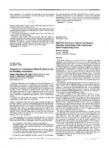
Fig. 1.
Constraint regions for example 1.
Example 1:
max (fl = -4x l + 2x 2 - 5x 3)
where x 2 solves
xl
max(f2 = -x 2 + 4x 3)
where x 3 solves
x2
max (f3 = 2x 3) x3
subject to 2x 2
-
x3 ~ 2
- 3x l + x 2
-
x 3 ~ -12
-3x 2
-
x 3 ~ -24 ~ 2
Xl 3
-x ~ -6 2
x ~ 0,
3
x ~
°
Fig. 1 displays S and the various inducible regions for this example. S2 is denoted by the hatched area and s' by the emboldened line. The global optimum occurs at point A and is listed along with a local optimum and their corresponding objective function values in Table I. Notice that the "high point" for this example, obtained by maximizing t' over S, occurs at D (see Table I); however, if player 1 were to select Xl = 2, players 2 and 3 would choose x 2 = 4 and x 3 = 6, respectively, yielding point B, a convenient lower bound on fl. Of further interest is the fact that the global optimum found at point A is dominated [2] by point E in that player 1 achieves a better result at E while the payoffs of the other two players remain the same. Thus, it can be seen that solutions to the MLPP need not be Pareto-optimal. This is a direct consequence of the operational assumption in multilevel programming that rules out cooperation among the players.
Ver tex
[1
[2
2 -163
-1
[3
Global Opt imun , A
14 (3,1,0)
Local Optimun, B
(2,4,6)
-30
20
12
Feasible Point , C
(~3' 4 , 6)
-3~
20
12
High Point, D
(2,8,0)
8
-8
Probl em (7) Sol ut ion, E
(2,1,0)
-6
-1
3
In general, the lack of an explicit sufficiency test to determine whether a trial point is in Sl is the major limitation that must be overcome if (1) is to be solved efficiently. Once a vertex is identified the bilevel program for the second player, given by (3), must then be solved. Although there are a number of algorithms that will perform these calculations (e.g., see [14]-[16], [22]), this requirement greatly increases the overall workload. Nevertheless, because this two step approach seems unavoidable, developmental efforts should concentrate on limiting the number of times (3) has to be solved. In [17] a grid search algorithm is proposed that begins by setting up a parameterized linear program whose solution for the" appropriate" choice of parameters coincides with that of (1). The objective function for the corresponding problem is formulated as a convex combination of the three objective functions given in (2)-(4). The weights are adaptively varied over the unit simplex by exploiting sensitivity information at each iteration. The principal limitation of this approach seems to be the bookkeeping burden imposed by the prospect of multiple optimal solutions. A second approach offered by Wen [22] combines the "K-Best" algorithm [15] to identify initial trial points, and a complementary pivot algorithm to test for bilevel optimality; i.e., inclusion in X 2 • The hybrid method begins by maximizing fl over S to obtain the high point, (Xl, x 2 , x3 ) , which is subsequently checked for feasibility by solving (3) with Xl fixed. If the resultant point is in X 2 the algorithm terminates with the global optimum; if not the "K-Best" vertex is found by examining adjacent extreme points. The feasible point which produces the largest value of fl under certain stopping conditions is declared the solution. Although this procedure seems to work satisfactorily for most problems, its computational load grows geometrically with the number of constraints. In addition, the usefulness of the complementary pivot algorithm may be limited when degeneracy is present. III.
NECESSARY CONDITIONS FOR THE
TLPP
Many of the algorithms developed for solving the BLPP are based on the realization that its inducible region can be represented exactly. In [8] it is shown that the follower's
714
IEEE TRANSACTIONS ON SYSTEMS, MAN, AND CYBERNETICS, VOL. SMc-14, No.5, SEPTEMBER/OCTOBER 1984
(Sd) (Se)
Theorem 1: For Xl fixed at x l * there exists a finite K such that (x 2*, x 3*, u*) solves (Sb)-(Sf) if and only if it solves (6b )-(6e). Proof: To find the appropriate K for the case where (x 2*, x 3*, u*) solves (Sb)-(Sf) let X = {I x )": Xl = x l*; i = 1,· .. , r} be the set of distinct vertices of (6c) and U = {(u)J: j = 1,· .. , p} be the set of distinct vertices of (6d)-(6e). From bilevel programming we know x* E X and u * E U, and from bilinear programming we know that a solution to (6b)-(6e) must be in X X U. If (6b) is now evaluated at each of the r X p vertices the complementarity term will either be positive or zero. For the latter case (x *, u *) clearly provides the largest payoff. Alternatively when u(A1x l + A 2x 2 + A 3x 3 - d) > 0, if K is selected such that
(Sf)
K> max (b 2 x 2
problem can be replaced by a system of inequalities derived from his Kuhn-Tucker conditions. A global solution to the resultant nonconvex, but differentiable program, provides the solution to the accompanying BLPP. Making use of this result an alternative to (1) is now offered: max I j" = alx l + a 2x 2 + a 3x 3 ) xl
where (x 2 , x 3 ) solves
tJ? = b
max
x2, x3,
2
x
2
+b
3
x
3
(Sa) (Sb)
)
U
subject to
A1x l
+ A 2x 2 + A 3x 3 uA
3
~ d =
-c
u ~ 0 u(Alx l
+ A 2x 2 + A 3x 3
d)
-
=
0
(Sc) 3
where u is an m-dimensional row vector of dual variables and (5d)-(5f) are the necessary conditions associated with the third player's problem. Notice that player 2 now has control over x 3 and u as well as x 2 • Due to the presence of the complementarity term (Sf), (5a)-(5f) is a nonlinear BLPP that resists solution in its current form. If player 1 is removed from the formulation by temporarily fixing Xl, however, (Sb)-(Sf) is easily solved through such techniques as branch and bound [14], complementary pivoting [22], or implicit enumeration [16]. Although it would be tempting at this stage to repeat the transformation used to obtain (S), the resultant problem, although offering an explicit approximation to SI, would be highly nonconvex and extremely difficult to solve globally. But even if such a solution were obtained, there would be no guarantee that it would fall in the level-two inducible region S2. This, of course, stems from the fact that the Kuhn-Tucker conditions associated with the inside problem (Sb)-(5f) for Xl fixed are only necessary; (Sf) precludes sufficiency. This situation appears to be unavoidable; however, the first difficulty can be .skirted by attaching an appropriately large weight to the complementarity term (5f) and then shifting it to the objective function (Sb), This leads to the following:
+ a 2x 2 + a 3x 3
max a1x 1
x 2 , x 3 .u
[b 2x 2+b 3x 3
subject to A1x 1 + A 2x 2
+ A 3x 3
~ d
uA 3 = -c 3 u ~
0
(6c) (6d) (6e)
where K is a sufficiently large finite constant. When Xl is fixed, (6b)-(6e) is essentially a bilinear programming problem whose solution occurs at a vertex of (6c)-(6e) [23]. We make use of this fact in the following theorem that establishes the equivalence of (5) and (6), and hence, (1).
+ b3x 3
b 2x 2 * - b3x 3 * ) j
-
u(Alx l*
+ A 2x 2 + A 3x 3
d)
-
the optimality of (x*, u*) would still be assured. Because b 2 x 2 + b 3x 3 is bounded above on (6c) the first part of the theorem follows. For the case where (x 2 *, x 3 *, u*) solves (6b)-(6e) we can pick the above K so this point must necessarily solve (Sb)-(Sf). The constraint region of (6) is a convex polytope and hence easier to work with then that of (S). In the following theorem we again appeal to the Kuhn-Tucker conditions of the inside problem to obtain an over approximation of the level-two inducible region. Theorem 2: A necessary condition that x* solves the linear TLPP is that there exists a u * E R m, U* E R"', and v* E R'" such that (x*, u", u*, v*) is feasible to
(7a)
x,u,u,v
subject to Alx l + A 2x 2 + A 3x 3 ~ d
(7b) (7c)
uA 3 = -c 3 u[A
2,A 3
Ku - v u(Alx l v(Alx l
xl
max
xiEX uJE U
]
= -[b
2,b 3
+ U= 0
]
(7d) (7e)
+ A 2x 2 + A 3x 3
-
d)
=
0
(7f)
+A
-
d)
=
0
(7g)
u ~ 0
(7h)
v ~ O.
(7i)
2x 2
+A
3x 3
Proof: A straightforward application of the KuhnTucker theorem to the inside problem of (6) with Xl fixed yields the desired result. The only complication arises from the stationarity term associated with u that is now shown to be redundant. Let v, vI, and v 2 be the m-dimensional Kuhn-Tucker multipliers associated with (6c)-(6e), respectively. First-order stationarity with respect to u yields - K(Alx l + A 2x2 + A 3x 3 - d) + A 3v l + I v 2 = 0 (8) m
where 1m is the m-dimensional identity matrix, and v 2 ~
o.
715
BARD: LINEAR THREE-LEVEL PROGRAMMING PROBLEM
In addition, complementarity requires that uv2 = o. If we now reintroduce the initial complementary term u(A 1x1 + A 2x 2 + A 3x 3 - d) = 0 into the formulation we can always set VI = 0 and v 2 = K(Alx l + A 2x 2 + A 3x 3 - d) to satisfy (8) identically. In a similar manner the above results can be readily extended to the p-Ievel problem by negatively weighting the two constraints (7f) and (7g), and placing them in the objective function. Each transformation requires the addition of a minimum of m variables (Kuhn-Tucker multipliers). Bookkeeping variables such as ii may be introduced for convenience. When example 1 is cast in the form of (7) with K = 100, we get the following results:
1° = (-6,
-1,0)
Xo
= (2,1,0)
Uo
= (2,0,0,0,0,0)
Uo = (0.5,0,0,0,3.5,0) V
o = (200.5,0,0,0,3.5,0).
Notice that x", depicted as point E in Fig. 1, is not in the level-one inducible region Sl so it cannot be the solution. In fact, as previously mentioned, when player 1 selects 2 3 Xl = 2, player 2 and 3 will choose x = 4 and x = 6 leading to the local optimum depicted as point B. Finally we see that while I l ( x ) = / 1( x o) = -6 is a supporting hyperplane of S, given by (7b), Il(x) = Il(x*) = -16i is not. Because this situation is generally true and, in particular, true at a nonglobal optimum, it will be exploited in the next section as part of the search algorithm. IV.
A
SIMPLEX-CUTTING PLANE ALGORITHM
The procedure that we propose for globally solving the linear TLPP combines simplexical vertex enumeration with the approximate program developed in Section III to selectively identify candidate solutions. The following lemma summarizes the properties of problems (1) and (7), and serves to underpin the algorithmic structure. Lemma: The objective function 11 evaluated at a solution to (7) provides an upper bound on the optimal value of the linear TLPP (4). b) A solution to (7) is always in the level-three rational reaction set X 3 ( x '. X2). c) The hyperplane I l( X) = I l( X*), where x * is a local solution to (1), supports the ·convex hull of the level-one inducible region sl, if and only if, x* is a global optimum. Algorithm: a)
Solve (7) to get the trial point, X, and a tight upper bound on 11. Step 2: Fix Xl at Xl and solve (3) to get (x )1. If X = (x )! or if Il(x)l = Il(x) stop; otherwise define /1 = Il(x)l as a lower bound and go to step 3. Step 1:
Step 3:
Step 4:
Step 5:
Search for a vertex adjacent to (x)" that both lies in the level-one inducible region Sl and is in the direction of increase of fl. If none is found go to step 4; otherwise move to this vertex and repeat the search until a local optimum is reached; call it x * and update the lower bound by setting /1 = Il(x*). Add the cut 11 ~ /1 + € to the constraint set of (7) and solve to get x. Here e > is a sufficiently small constant chosen so that no unexplored vertices of S are eliminated. Test to see whether x is in Sl by fixing Xl at Xl and solving (3). If the test is positive put (x) k + 1 = X, eliminate the cut and go to step 3; otherwise search adjacent vertices in the direction of increase for a point (X)k+l in Sl. Repeat search if necessary starting from each of the other multiple solutions obtained at step 4 until such a point is found; then go to step 3. If the search fails stop with x* as the global optimum.
°
The algorithm is designed to take advantage of the connectedness of the level-one inducible region sl, and the fact that the solution to (1) must occur at a vertex of S. At step 1, a convenient starting point is found and subsequently tested for global optimality at step 2. Termination occurs if either x is in S 1 or (x)', which is in S 1 by construction, yields an objective function value equal to the upper bound derived by solving (7). At step 3 a simplex-type search is conducted over Sl to arrive at a local optimum. This requires that before a vertex be included along the path of increase, problem (3) be solved to assure its membership in s'. Next a cut is added to remove the incumbent solution from the constraint region. Parraga [18] used a similar procedure in his approach to the BLPP. Another trial point, which in general will not be a vertex of S or even an element in S\ is then obtained by resolving (7). However, we see from part c) of the lemma, that if the current local optimum is not the global optimum, the cut will intersect the level-one inducible region; step 5 is designed to find a point of intersection. The search is facilitated by the parallel nature of the cut that permits the ready identification of potential elements of the level-two rational reaction set X 2 • This can be achieved by pivoting through the multiple optimal solutions present when (7) is solved. The actual procedure implemented was based on the work of Mattheis [24]. When the algorithm is applied to example 1, step 1 produces the point x = (2, 1, 0) that is seen in Fig. 1 not to lie in Sl. Upon fixing Xl at 2 and solving the inside problem (3) we get the point B, which happens to be an element of Sl. The search at step 3 leads to the conclusion that this point, (x)! = (2, 4, 6) is a local solution x * because there are no adjacent vertices that both lie in Sl and are in a direction of increase. At step 4, the cut - 4x l + 2x 2 - 5x 3 ~ - 30 + € is added to the constraint region and (7) resolved to give a new x = (4.57,6.43,4.71). Here, € was chosen as 1. The point x lies along the edge FG and
716
IEEE TRANSACTIONS ON SYSTEMS, MAN, AND CYBERNETICS, VOL. SMc-14, No.5, SEPTEMBER/OCTOBER 1984
is not in SI; therefore, at step 5 a search of adjacent vertices must be conducted to find an element of the level-one inducible region that intersects the cut, should one exist. The search leads to the point (X)2 = (3.65,3.05,4.1) that lies along the edge AC. Returning to step 3 brings us to point A, which turns out to be the local optimum x* = (14/3,1,0). A second cut must now be added but the algorithm terminates at step 5 when no new point in SI can be found that produces a value of /1 larger than -161, the best lower bound. V.
COMPUTATIONAL EXPERIENCE
Although a fully automated code is still under development, the algorithm has been tested on a limited set of problems. In each formulation, input parameters included the individual number of level variables and the total number of structural constraints. Nonnegativity of the decision variables was assumed throughout the analysis. In all, 21 problems were solved ranging in size from seven variables and seven constraints to 24 variables and 27 constraints. The procedure discussed in [14] was used to solve the subproblems given by (7). The results are summarized in Table II for the three distinct cases investigated. Algorithmic performance was measured by the following statistics: the average number of cuts needed at step 4; the average number of bilevel programming problems (BLPP) solved, primarily at steps 4 and 5; the average number of simplex-type pivots required to find a point inS 1, the level-one inducible region, at steps 3 and 5; and the average CPU time (all computations were performed on a VAXll-780). From .Table II it can be seen that the number of cuts required seems to grow linearly with the problem size (as measured by the number of constraints, m), while the computational burden (as measured by the number of subproblems that must be solved) appears to grow at a rate slightly less than the square of m. This has serious implications for problems of large scale; however, it should be noted that .because the cuts introduced at step 4 for the purpose of locating new points in SI are only temporary (being removed as step 5), the dimensions of the BLPP's that must be solved in the course of the algorithm remain unchanged. More efficient solutions to the former should therefore greatly reduce the overall amount of numerical work. With regard to CPU time, the basic results compare favorably to those of Wen [22] who used the much faster CDC Cyber in his analysis. Finally, despite the fact that the adjacent vertex search at step 3 is conceptually quite tedious, it can be performed quickly and efficiently in a tableau format, and thus does not represent a major hurdle to implementation. VI.
SUMMARY AND CONCLUSION
A model has been presented that attempts to capture the way in which decisions are made in hierarchical noncooperative systems. In the development, Stackelberg concepts relating to the inducible region and the rational reaction
TABLE II COMPUTATIONAL EXPERIENCE
Data In put th. tb. tb.
Par ame te r s: 1 2 3 of Variables (n t n t n ) of Constraints* (rn) of Test Problems
Output Results: Average tb. of Olts/Problems Average tb. of Pivots/Cuts Average l'b. of BLPPs SoLv ed Average CPU Time (minutes)
Case I
Case II
Case III
(2,2,3) 7 10
(4,5,5) 15 6
(6,9,8) 27 5
9.6 13.5 18.8 1. 07
41.2 38.3 2.32
4.3 6.4 5.7 0.37
16.9
*I:bes not include nonnegativity of the decision variables.
set have been extended to the three-level open-loop game. A disturbing feature of the resulting solution, though, is that it may not be Pareto-optimal. As a consequence some players may be assigned payoffs inferior to what they would have realized had another analytical approach been used. Nevertheless, when decisions are made sequentially by persons who are either forbidden to communication (such as government regulators and industrial planners, perhaps), or find it disadvantageous to cooperate (such as lower level managers in a decentralized firm), the multilevel programming model may be appropriate. To this end, a cutting plane algorithm has been developed to solve the linear three-level case. The algorithm takes advantage of both a basic geometric property of the problem that assures that under fairly general conditions a solution will occur at the vertex of the underlying constraint polyhedron, and a set of first order necessary conditions derived from standard programming considerations. The principal computational steps involve solving a BLPP and enumerating adjacent vertices at each iteration. Although it is still too early to say how well the algorithm will perform on large-scale problems, results for a limited number of test cases suggest that problems with up to 100 variables and 100 constraints are well within the manageable range. Improvements in the actual code should also yield greater computational efficiencies. REFERENCES
[1] R. L. Keeney and H. Raiffa, Decisions with Multiple Objectives: Preferences and Value Trade-offs. New York: Wiley, 1976. [2] M. Zeleny, Multiple Criteria Decision Making. New York: MeGraw-Hill, 1982. [3] K. Tarvainen and Y. Y. Haimes, "Coordination of hierarchical multiobjective systems: Theory and methodology," IEEE Trans. Syst., Man, Cybern., vol. SMC-7, no. 3, pp. 125-143, 1977. [4] A. M. Geoffrion, "Proper efficiency and the theory of vector maximization," J. Math. Anal. and Applicat., vol. 22, pp. 618-630, 1968. [5] R. E. Wendell, "Multiple objective mathematical programming with respect to multiple decision-makers," Oper. Res., vol. 28, no. 5, pp. 1100-1111, 1980. [6] W. Davis and' J. Talvage, "Three-level models for hierarchical coordination," Omega, vol. 5, no. 6, pp. 709-720, 1977. [7] E. P. Winkofsky, N. R. Baker and D. J. Sweeney, "A decision process model of R&D resource allocation in hierarchical organizations," Management Sci. vol. 27, no. 3, pp. 268-283, 1981. [8] J. F. Bard, "Coordination of a multidivisional organization through
IEEE TRANSACTIONS ON SYSTEMS, MAN, AND CYBERNETICS, VOL. SMc-14, NO.5, SEPTEMBER/OCTOBER 1984
[9] [10] [11] [12]
[13] [14] [15] [16]
two levels of management," Omega, vol. 11, no. 5, pp. 457-468, 1983. J. Nash, "Non-cooperative games," Annals of Math., vol. 54, pp. 286-295, 1951. M. Simaan and J. B. Cruz, Jr., "On the Stackelberg strategy in nonzero-sum games," J. Optimization Theory and Applicat., vol. 11, pp. 533-555, 1973. J. E. Falk, "A linear max-min problem," Math. Program., vol. 5, pp. 169-188, 1973. T. S. Chang and P. B. Luh, "Derivation of necessary and sufficient conditions for single-stage Stackelberg games via the inducible region concept," IEEE Trans. Automat. Contr., vol. AC-28, no. 8, 1983. B. F. Gardner and 1. B. Cruz, Jr., "Feedback Stackelberg strategy for M-Ievel hierarchical games," IEEE Trans. Automat. Contr., vol. AC-23, no. 3, pp. 489-493, 1978. J. F. Bard and J. E. Falk, "An explicit solution to the multi-level programming problem," Computers and Operations Research, vol. 9, no. 1, pp. 77-100, 1982. W. F. Bialas and M. H. Karwan, "On two-level optimization," IEEE Trans. Automat. Contr., vol. AC-27, no. 1, pp. 211-214, 1982. W. Candler and R. Townsley, "A linear two-level programming problem," Computers and Operations Research, vol. 9, no. 1, pp.
717
59-76, 1982. [17] J. F. Bard, "Optimization in multilevel systems," in Proc. American Control Conf., vol. 1, Arlington, VA, 1982, pp. 403-408. [18] F. Parraga, "A methodology of interceptions for the solution of the two-level hierarchical problem with linear objectives," Ph.D. dissertation, Systems and Industrial Engineering Dept., Univ. Arizona, Tucson, 1980. [19] T. Basar and H. Selbuz, "Closed loop Stackelberg strategies with applications in optimal control of multilevel systems," IEEE Trans. Automat. Contr., vol. AC-24, no. 2, pp. 166-178, 1979. [20] M. S. Mahoud, "Multilevel systems control and applications: A survey," IEEE Trans. Syst., Man, Cybern., vol. SMC-7, no. 3, pp. 125-143,1977. [21] J. F. Bard, "Optimality conditions for the bilevel programming problem," Naval Research Logistics Quart., vol. 31, pp. 13-26,1984. [22] U. P. Wen, "Mathematical methods for multilevel linear programming," Ph.D. dissertation, Dept. Industrial Engineering, State University of New York, Buffalo, 1981. [23] H. Vaish and C. M. Shetty, "The bilinear programming problem," Naval Research Logistics Quart., vol. 23, pp. 303-309, 1976. [24] T. H. Mattheiss, "An algorithm for determining irrelevant constraints and all vertices in systems of linear inequalities," Oper. Res., vol. 21, no. 1, pp. 247-260, 1973.
An Information Channel Model of a Neuron Encoder and Possible Microwave Radiation Effects on Capacity WILLIAM D. O'NEILL AND JAMES C. LIN
Abstract-A popular neuron encoder model is cast into the form of an information channel and the encoder state is shown to be measured in probability by a Markov chain. Channel capacity of the model is calculated under the assumption that the neuron threshold is approximately Gaussian distributed. The model is also shown to be characterized in information theory terms as a finite-state indecomposable channel subject to intersymbol interference and fading. From experiments on snail neurons, which were the stimulus for our modeling efforts, the hypothesis is suggested that, to the extent our model captures the actual performance of neurons, microwave radiation could significantly alter the information processing ability of neurons.
I.
INTRODUCTION
I
N FORMATION modeling of neurons began almost immediately after the recognition that a neuron could be considered an information channel in the Shannon sense Manuscript received January 19, 1983; revised October 1983, February 1984, and April 1984. This work was supported in part by the National Science Foundation and the Office of Naval Research. W. D. O'Neill is with the Department of Industrial and Systems Engineering and the Department of Bioengineering, University of Illinois at Chicago, Chicago, IL 60680. J. C. Lin is with the Department of Bioengineering, University of Illinois at Chicago, Chicago, IL 60680.
[1], [2]. An excellent and comprehensive review of these efforts up to 1976 can be found in [3]. Since 1976 studies have focused primarily on more sophisticated experiments and analysis but have not strayed far from the models proposed by Stein et al. [4]. A smaller body of literature concerns itself with multiple neuron models [5]-[7]. Recent efforts display a wide variety of types of neurons, some within networks, but all still maintain a common characteristic of considering the analysis of the neuron in toto- from postsynaptic inputs through the cell body to the axon, and from these to the post synaptic input of the next neuron [8]-[10]. A distinguishing feature of this study is that the analysis will consider only the neuron encoder and will derive a detailed information channel model of this component of the neuron. A schematic neuron illustrating itscomponents is shown in Fig. 1. The multiple input signal source provides a source of slowly varying dendritic currents into the cell body. The spike generating mechanism of the cell produces an action potential when the cell threshold is exceeded. Such potentials are propagated along the axon to the synaptic decoder whereupon they contribute to the
0018-9472/84/0900-0717$01.00 ©1984 IEEE