download from http://www.victoria.ac.nz/raman/publis/codes/cobra.aspx. Index Headings: Wavelet transform; Background subtraction; Raman spectroscopy ...
An Iterative Algorithm for Background Removal in Spectroscopy by Wavelet Transforms C. M. GALLOWAY,* E. C. LE RU, and P. G. ETCHEGOIN The MacDiarmid Institute for Advanced Materials and Nanotechnology, School of Chemical and Physical Sciences, Victoria University of Wellington, PO Box 600 Wellington, New Zealand
Wavelet transforms are an extremely powerful tool when it comes to processing signals that have very ‘‘low frequency’’ components or nonperiodic events. Our particular interest here is in the ability of wavelet transforms to remove backgrounds of spectroscopic signals. We will discuss the case of surface-enhanced Raman spectroscopy (SERS) for illustration, but the situation it depicts is widespread throughout a myriad of different types of spectroscopies (IR, NMR, etc.). We outline a purposebuilt algorithm that we have developed to perform an iterative wavelet transform. In this algorithm, the effect of the signal peaks above the background is reduced after each iteration until the fit converges close to the real background. Experimental examples of two different SERS applications are given: one involving broad backgrounds (that do not vary much among spectra), and another that involves single molecule SERS (SM-SERS) measurements with narrower (and varying) backgrounds. In both cases, we will show that wavelet transforms can be used to fit the background with a great deal of accuracy, thus providing the framework for automatic background removal of large sets of data (typically obtained in time-series or spatial mappings). A MATLABt based application that utilizes the iterative algorithm developed here is freely available to download from http://www.victoria.ac.nz/raman/publis/codes/cobra.aspx. Index Headings: Wavelet transform; Background subtraction; Raman spectroscopy; Data processing; Surface-enhanced Raman spectroscopy; SERS.
INTRODUCTION There are many situations in spectroscopy where background removal is necessary. Our specific interests lie in surface-enhanced Raman spectroscopy (SERS), but there are many other spectroscopic applications (such as nuclear magnetic resonance (NMR), electron paramagnetic resonance (EPR), or infrared (IR) spectroscopy) where the separation of the background and signal peaks are important. Arguably the most important feature of any background removal algorithm is its ability to operate efficiently with minimum user intervention. This then allows the removal of the background from a very large number of spectra without having to adjust parameters for each, for example, when performing time series measurements or spatial mappings in Raman, SERS, or related techniques. From an analytical point of view, a situation very often found (for example in Raman scattering) is the following: we would like to know the composition of a sample in different places (in a mapping, for example) in terms of a number of reference compounds for which we know the bare (background-less) spectra. The best way to quantify this is by a linear decomposition of a given spectrum of the sample in terms of the known reference spectra. This method works well if the spectra we are trying to quantify do not contain spurious Received 28 May 2009; accepted 3 September 2009. * Author to whom correspondence should be sent. E-mail: chris.gallow@ gmail.com.
1370
Volume 63, Number 12, 2009
backgrounds (from impurities or additional compounds). If the background is very similar from point to point in the mapping, a relatively easy background subtraction for all of them could be achieved before the linear decomposition in terms of the reference spectra is performed. However, if the background changes randomly from point to point, a more reliable and efficient background subtraction routine is needed: one that will not introduce artifacts in the process of subtracting the background and that can be carried out for hundreds (sometimes thousands, or tens of thousands) of spectra. A few tens of spectra can be analyzed by hand, but it is unlikely that tens of thousands of spectra (in a Raman map or a time series, for example) can be analyzed in this way. SERS spectra (and single molecule (SM) SERS in particular, to which this application is particularly suited) are particularly susceptible to randomly occurring backgrounds from event to event in either mappings or time series (in colloidal liquids).1 For resonant or pre-resonant dye molecules, these backgrounds can be attributed to surface-enhanced fluorescence,2 whose spectral profile is modified by the underlying plasmon resonance dispersion.3 The combination of large numbers of spectra and unpredictable backgrounds makes it desirable to have an analysis tool of the type described hitherto. It is the type of problem described above that has led us to develop a technique that utilizes wavelet transforms (WT)4–7 for the automatic background removal of large numbers of spectra. In the past, WTs have been used for many signal processing applications including de-noising,8,9 spike removal,8 and background removal10,11 (including also Raman applications9,10,12). However, we have improved here the ability of wavelet transforms to remove backgrounds by using an iterative process of signal modification (explained later in the Iterative Wavelet Transform Algorithm section). Techniques based on wavelet transforms for background removal, in which there is a substantial difference between the frequency domain of the analytical signal and the background, have been investigated in the past.13 Many of our interests, however, lie in areas where there is not such an obvious difference. In fact, there may be cases where there is an overlap between the frequency regimes and additional adjustments to the wavelet transform need to be performed in order to obtain the most accurate background fits. The algorithm is implemented and provided in a MATLABt-based application (along with a manual) that can be used for background removal and noise reduction of a large number of spectra; it is freely available from our website.14
BACKGROUND REMOVAL USING WAVELET TRANSFORMS It is not uncommon in signal processing to be working with spectra that contain three main characteristic sources, having
0003-7028/09/6312-1370$2.00/0 Ó 2009 Society for Applied Spectroscopy
APPLIED SPECTROSCOPY
FIG. 1. An example SERS spectra of a common probe (rhodamine 6G: RH6G), highlighting the different typical ‘‘frequency’’ regimes encountered in many type of spectroscopies: the ‘‘high-frequency’’ noise, the ‘‘mediumfrequency’’ SERS peaks, and the ‘‘low-frequency’’ background.
particular frequency regimes and representing different main features of the data (see Fig. 1 for an example of a SERS spectrum): high frequency noise, medium frequency signal peaks, and a low frequency background. We shall give first a brief technical account of the overall situation, even though this is not necessary to understand how to use our algorithm in practice. A significant amount of research has been performed on how wavelet transforms can be used for background removal often involving decomposing the signal until both the noise and signal peaks have been removed in the detail coefficients. However, this is only accurate when the frequency domain of the peaks and background are distinguishable. In the Fourier domain, a wavelet has the shape of a band pass filter. As a result, each detail level contains the components of the signal that lie within a certain frequency range defined by the type of wavelet used and the scale at which it is performed. In order to separate the signal from the peaks and noise from the raw data without modifying the background, the frequency domain of the background must be in a region that does not contain any contribution from the peaks or noise. If this is the case—at a sufficiently large decomposition level—only the background contribution will remain in the approximation coefficients. By reconstructing the signal using only the approximation coefficients (also known as an approximation curve or spectrum), an accurate background fit can be achieved. Nevertheless, it is often the case in spectroscopy that there will be an overlap in the frequency region of the peaks and the background. Consequently, performing the decomposition until the signal peaks are removed will also remove some of the background contribution from the approximation coefficients. It is therefore impossible to obtain an accurate background fit directly from the wavelet coefficients. In this paper we will address this problem by proposing a new algorithm for the removal of backgrounds from signals with overlapping frequency regions (typical of spectroscopies such as Raman).
THE ITERATIVE WAVELET TRANSFORM ALGORITHM The iterative wavelet transform algorithm is based around the concept of modifying the signal depending on the wavelet coefficients obtained from the discrete wavelet transform (DWT) decomposition. Even though we cannot separate the
FIG. 2. The same spectrum shown in Fig. 1 undergoing ten iterations of DWT background fits. (a) The original signal and the 7th level approximation curve after a single iteration. Notice that the approximation spectrum is not really a good representation of the real background (due to the presence of the SERS peaks). The signal is therefore modified as shown in (b), so that all points above the approximation spectrum are set equal to the approximation spectrum itself. The SERS peaks are then chopped at the approximation curve level and a new DWT is then performed (on the modified signal) up to the 7th level. The new approximation curve is also plotted in (b). The process is then repeated, and after each iteration the effect of the SERS peaks on the background fit is reduced, until it finally converges to the most physical representation (without including the peaks) as shown in (c). The exact number of iterations needed for the fit to converge will typically depend on the size of the peaks and how closely spaced they are. This can be decided on a case-by-case basis according to the spectra being analyzed.
background contribution from the peak contribution, we can decompose the signal to a level where all of the background is only just contained within the final set of approximation coefficients. The approximation spectrum is then reconstructed, resulting in a curve that is close to a background fit but slightly modified due to the peak contribution remaining in the
APPLIED SPECTROSCOPY
1371
FIG. 3. A simulated spectrum of 1024 data points and consisting of a thirdorder polynomial background, Gaussian shaped signal peaks, and random noise. To test the capabilities of the algorithm we have included a relatively wide peak close to ;1500 cm 1 and a collection of three peaks around ;1200 cm 1.
coefficients (see Fig. 2a). If the original signal is then modified by taking all points above the fit and setting them equal to it, we can re-perform the decomposition to the same level with the modified signal and obtain a slightly more accurate background fit (see Fig. 2b). The reason for this is that the signal contribution in the frequency region of the background has been lessened due to the reduction in the peak intensities. This process of decomposition and signal modification can be repeated until the fit converges (see Fig. 2c), which should occur when all of the peak contribution has been removed from the approximation coefficients. The final fit will then be very close to the real (physical) background. Often there will be situations where the fit will be below the signal in regions that are obviously purely background. Typically this will occur close to the boundaries, but there may be additional regions, close to a large group of closely packed peaks for instance. In these situations it is useful to define regions that the algorithm can assume are purely background and will never be modified. How critical the background regions are will be investigated in the remaining sections of the paper. Once the number of decomposition levels has been defined, along with the iteration number and wavelet type, the background removal can be applied to many spectra without modifying the parameters, as long as the defined background regions are relevant for all cases. The best results will be achieved if the algorithm parameters are estimated on the signal event with the highest frequency background, as the decomposition level depends only on the frequency of the background and not on the overall shape. The remainder of the paper will be dedicated to investigating the accuracy of the background fit using the iterative algorithm.
A SIMULATED SIGNAL In order to ascertain the accuracy of the background fit, we need a signal in which we actually know the real background. We have therefore chosen as our first example a simulated spectrum of 1024 points (same as a typical charge-coupled device (CCD) readout), which has a background defined by a third-order polynomial, peaks that have a Gaussian line shape,
1372
Volume 63, Number 12, 2009
and random noise. Figure 3 shows the simulated signal and the real background. To test the accuracy of the iterative algorithm and the effect of defining background regions, the background fit is performed in six different ways. In each case we have chosen to use the Daubechies 10 wavelet and the iterative algorithm is performed for 10 iterations. This is typically enough to get convergence of the background fit for most cases. Figure 4 shows the six different background fits, along with Table I, which contains the parameters and their accuracy. Figures 4a through 4d consist of fits using the iterative algorithm, while Figs. 4e through 4f have fits that use the approximation spectrum before any signal modification is performed. The best fit occurs using the iterative algorithm with a decomposition level of 6, but with all of the background regions defined (see Fig. 4b). This is not surprising as only the peaks will be modified after each iteration. Often it is not possible, however, to define this many background regions. If we restrict ourselves to only defining the background at the boundaries, but keep the decomposition level the same (see Fig. 4a), the fit is greatly distorted close to the peaks, in particular, close to the group of three peaks at ;1200 cm 1 and the wider peak at ;1500 cm 1. Increasing the decomposition level to 7 (see Fig. 4c) significantly reduces the distortion, but there is still a region close to ;1500 cm 1 where the fit drops below the signal. Defining a third background region on the right hand side of the ;1500 cm 1 peak corrects this. If we compare these fits with what is expected without the iterative process of signal modification (see Figs. 4e and 4f), we can see that the iterative algorithm outperforms the conventional choices. In particular, by comparing the fits in Figs. 4c and 4e, we can see the advantage of the iterative algorithm. Both fits have a decomposition level of 7 in the DWT, but the former case goes through 10 iterations of signal modification while there is none in the latter. It is obvious in the second case that the signal peaks have a significant contribution to the fit. Increasing the decomposition level to 8 meant that the non-iterated fit was significantly better (see Fig. 4f) but not as good as what could be achieved with the iterative algorithm. By looking at the v2 values in Table I, one might assume that the accuracy of the fit is independent of the decomposition level. But if we actually look at the fits in Figs. 4a and 4c it is obvious that the latter is a much better representation of the background. In the former case, the fit is very close to the real background but with slight distortions close to the peaks that will lead to incorrect estimates of the peak properties (the peak intensity, for example). The latter case, however, follows the actual background quite closely but with a significant distortion close to the ;1500 cm 1 peak. This was corrected by defining a third background region to help in the convergence of the algorithm.
EXAMPLES FROM REAL DATA: SURFACEENHANCED RAMAN SPECTROSCOPY WITH BACKGROUNDS OF VARYING INTENSITIES The second example looks at how the SERS peaks and underlying fluorescence intensities change as the SERS probe is moved closer to or further away from a SERS-active substrate by means of an electric field.15 In this case, the background is relatively broad and its shape remains similar from one spectrum to the other; only its intensity (relative to the peaks) varies. What makes the separation of Raman peaks
FIG. 4. The simulated spectrum shown in Fig. 3 with six different types of wavelet-based background fits with the fitting parameters defined in Table I. (a–d) are fitted using the iterative algorithm while (e) and (f) are fitted with the non-iterative approximation curve. In all cases the solid black curve represents the ‘‘real’’ background, while the dashed black lines are the fitted versions. Note the superiority of the fit in (b) with respect to all other cases (see Table I for complementary information on the different fits).
from the fluorescence important in this experiment is their different origins. The full details of this study and its physical interpretation can be found in Ref. 15. We only focus here on the background removal process of the data. Using our background removal program it was possible to obtain an accurate fit to the background and subtract it from the original spectra as shown in Fig. 5. This was carried out automatically on a large number of spectra (721 spectra as a function of time). Because the ‘‘frequency components’’ of the background signal are similar for all of the spectra, the choice of reference TABLE I. The fitting parameters used for the background fits in Fig. 4, as well as the v2 values for the difference between the real background and the fit in each case. Fit parameters Plot
Scale level
Iterations
Background regions
v2
a b c d e f
6 6 7 7 7 8
10 10 10 10 0 0
2 All 2 3 NB NB
435 120 426 279 1111 980
spectrum for determining the fitting parameters was not important. The wavelet transformation was performed at a decomposition level of 6. Furthermore, the background before the first Raman mode and after the last one was all that was required to achieve an accurate fit for all cases (due to the broadness of the background). We have also plotted in Fig. 5 the background fits that would be obtained from the approximation spectrum without any signal modification and a decomposition level of 7. Unsurprisingly, the difference between the two fits becomes more pronounced as the peak intensities become larger. It is obvious, however, that the iterative algorithm greatly improves the accuracy of the background fit.
ANOTHER SURFACE-ENHANCED RAMAN SPECTROSCOPY EXAMPLE: SINGLEMOLECULE SURFACE-ENHANCED RAMAN SPECTRA Notwithstanding, there are other more complicated background subtraction situations faced in SERS experiments (which are taken here as an archetypal example), in which there is not only a variation in the overall intensity but also in the spectral shape. This is the case in single-molecule SERS experiments of resonant or pre-resonant molecules.
APPLIED SPECTROSCOPY
1373
FIG. 5. The original spectra, background fits, and filtered spectra for three different cases; after Ref. 15. Two background fits are performed, one using the iterative algorithm and a decomposition level of 6 (solid black line), and one using the approximation spectrum without the algorithm and with a decomposition level of 7 (dashed black line). In this application of the algorithm, the shape of the fluorescence background does not change significantly over spectra, but the overall intensity does. See Ref. 15 for the actual experimental details. The ‘‘filtered’’ SERS spectra on the right can be analyzed subsequently without any interference from fluorescence.
When observing ensembles of molecules in SERS, the fluorescence background is typically broad and its overall shape does not change by a great deal when focusing the laser in a new location. On the contrary, in recent years there has been a lot of interest in single-molecule measurements in SERS16 and, as it turns out, the backgrounds can change rapidly from spectrum to spectrum (in both intensity and shape) due to the fact that they are not washed out by ensemble averaging over a large number of molecules. Single-molecule SERS spectra can reveal individual plasmon resonance dispersions of small clusters, affecting the surface-enhanced fluorescence emitted by the molecules,3 thus producing constantly varying shapes in the background signals underneath the SERS spectra.17 We therefore choose as our second example some recent measurements we have performed that look at how the fluorescence background and Stokes SERS intensities vary (relative to each other) for single-molecule SERS events.18 The analysis of thousands of such spectra is typically required in such a study. Even though it is not relevant for the present purposes here, we mention in passing that the aim of this experiment was to measure non-radiative effects that modify the Stokes and fluorescence intensities differently.18 The selected spectra in Fig. 6 of Crystal Violet (CV) have very different backgrounds but were all fitted with the same
1374
Volume 63, Number 12, 2009
parameters in the iterative DWT algorithm. The frequency components that dominated the background can vary quite significantly depending on the local environment of the molecule being observed and the particular plasmon resonance affecting it. However, a decomposition level of 6 was sufficient for the algorithm to obtain accurate background fits. Additionally, defining several background regions (including a region in between two Raman peaks) assisted with the convergence. This is not required for lower frequency backgrounds, such as the ones of the previous example. We have also plotted the background estimation using a decomposition level of 7 but without using the iterative algorithm. Again we see that the signal peaks greatly modify the expected background. Other measurements using rhodamine 6G (RH6G) instead of CV (see Fig. 7), which has a dense region of modes from ;1100 cm 1 to ;1650 cm 1, have also been investigated and can also be fitted with a great deal of accuracy. In this case a background region needed to be defined on each side of the dense region to obtain the best convergence of the fit. Furthermore, the dense region of peaks meant that the best fit was achieved at a decomposition level of 7 (compared with 6 in the case of CV, which has conveniently spaced peaks). We believe the examples presented here prove the point that automatic background subtraction (in the presence of randomly
FIG. 6. Spectra of Crystal Violet (CV) single-molecule SERS events with very different fluorescence backgrounds, and background fits using the iterative algorithm (solid black line) and the original approximation 7 spectrum (dashed black line). The plasmon resonance favors the: (a) high energy modes, (b) and (c) medium energy modes, and (d) low energy modes. The algorithm parameters were the same for all four cases, with the wavelet transform performed to the 6th level and 10 convergence iterations. The background was defined as comprising the regions: before the 440 cm 1 peak, after the 1620 cm 1 peak, and a small section between the 440 cm 1 and 800 cm 1 peaks. This is enough for the iterative algorithm to reliably find the background all the time for all spectra, thus allowing the automatic background subtraction of the very large numbers of spectra (.1000) needed to gain reliable statistics in SM-SERS conditions for this particular experiment.
occurring background shapes) is possible with the iterative DWT algorithm presented in this paper. This provides us then with a robust tool with which thousands of spectra can be analyzed automatically and reliably.
most accurate results from the MATLABt application provided with this paper:14 �
CONCLUSION Using an iterative process of DWT we have shown that it is possible to perform an accurate background removal for signals that may have an overlap in the frequency regions of the peaks and background. There are several important practical considerations that need to be made in order to obtain the
�
FIG. 7. A single molecule event of RH6G with a background fitting using the iterative algorithm at a decomposition level of 7 and background regions defined at the boundaries and on each side of the dense region of peaks that span the region 1100 cm 1 to 1700 cm 1.
The most important parameter that needs to be set is the scale level into which the signal will be decomposed. The higher the scale level is, the lower the background fit frequencies will be. Another way to state this is that at high scale levels, the ability of the background to ‘‘squeeze’’ into the signal peaks will decrease. However, if the level is set too high, then even the background will fluctuate too rapidly for an accurate fit to be made. Exactly which value to set will typically depend not on the background but on the shape of the signal peaks. For narrow peaks that are widely spaced out, we can go to relatively low scale levels and still get an accurate background. However, if the peaks are wide and/or close together, then we must decompose the signal to a larger scale. This is fine when the background is quite broad (as in the case of the ensemble SERS measurements in the Examples from Real Data section) but if it fluctuates quite rapidly (like in the single molecule measurements in the Another SERS Example section) then it may be necessary to define several background regions to assist with the fitting. This was, indeed, explicitly done in the data in Figs. 6 and 7. The number of iterations is also an important parameter, but not one that varies by a large amount between signals with different background frequencies. It may, however, depend on how large the signal peaks are compared to the background. Most of the spectra we looked at have similar Raman-to-background ratios, and hence the iteration number will not change very much. But in other potential uses of the algorithm we may have larger signal-to-background ratios and it may be needed to test how many iterations are required
APPLIED SPECTROSCOPY
1375
�
for convergence. This can easily be achieved by taking a single event and increasing the number of iterations in steps until further increases do not improve the final result. The final parameter that is of significant importance is the type of wavelet used for the DWT. In all of these examples we have used the Daubechies 10 wavelet,4–7 and this choice turns out to provide satisfactory results. We have tried several other types of wavelets and have always found that the higher level ones (i.e., more complicated) achieve the best results. However, there may be problems that require wavelets with a certain symmetry (or shape) and those may be better solved with something other than Daubechies wavelets. The wavelet type is, undoubtedly, something that needs to be decided for each specific application of the algorithm. We are confident to claim, however, that most problems dealing with spectroscopic signals similar to Raman spectra will find the Daubechies wavelets to be a very good option.
Overall we hope that the algorithm developed here and the program that can be freely downloaded from Ref. 14 will help other researchers to analyze their data and reach conclusions— that could not have been obtained otherwise—on the nature of the signals or the backgrounds over very large sets of data typical of modern spectroscopic applications (where automation of the analysis is most often necessary). ACKNOWLEDGMENTS P.G.E. and E.C.L.R. acknowledge partial support for this research by the Royal Society of New Zealand (RSNZ), through a Marsden Grant. We are indebted to Paul Lacharmoise (Institut de Cie`ncia de Materials de Barcelona–
1376
Volume 63, Number 12, 2009
CSIC, Spain) for providing unpublished data on ‘‘guiding molecules with electrostatic forces in SERS’’ (from the study in Ref. 15), and to Matthias Meyer (Victoria University of Wellington, New Zealand) for his assistance with the programming of the background removal application in MATLABt.
1. E. C. Le Ru, M. Meyer, and P. G. Etchegoin, J. Phys. Chem. B 110, 1944 (2006). 2. E. C. Le Ru, P. G. Etchegoin, J. Grand, N. Felidj, J. Aubard, and G. Levi, J. Phys. Chem. C 111, 16076 (2007). 3. E. C. Le Ru, J. Grand, N. Felidj, J. Aubard, G. Levi, A. Hohenau, J. R. Krenn, E. Blackie, and P. G. Etchegoin, J. Phys. Chem. C 112, 8117 (2008). 4. I. Daubechies, IEEE Trans. Info. Theory 36, 961 (1990). 5. M. Misiti, Y. Misiti, G. Oppenheim, and J. Poggi, Wavelet ToolboxTM 4 User’s Guide (The MathWorks, Inc., Natick, MA, 2008). 6. B. Walczak, Wavelets in Chemistry (Elsevier Science, Amsterdam, 2000). 7. A. K. Leung, F. Chau, and J. Gao, Chemom. Intell. Lab. Syst. 43, 165 (1998). 8. F. Ehrentreich and L. Summchen, Anal. Chem. 73, 4364 (2001). 9. W. Cai, L. Wang, Z. Pan, J. Zuo, C. Xu, and X. Shao, J. Raman Spectrosc. 32, 207 (2001). 10. P. M. Ramos and I. Ruisanchez, J. Raman Spectrosc. 36, 848 (2005). 11. L. Shao and P. R. Griffiths, Environ. Sci. Technol. 41, 7054 (2007). 12. Y. Hu, T. Jiang, A. Shen, W. Li, X. Wang, and J. Hu, Chemom. Intell. Lab. Syst. 85, 94 (2007). 13. H. Tan and S. D. Brown, J. Chemom. 16, 228 (2002). 14. http://www.victoria.ac.nz/raman/publis/codes/cobra.aspx. 15. P. D. Lacharmoise, E. C. Le Ru, and P. G. Etchegoin, ACS Nano3 3, 66 (2009). 16. P. G. Etchegoin and E. C. Le Ru, Principles of Surface-Enhanced Raman Spectroscopy and Related Plasmonic Effects (Elsevier, Amsterdam, 2009). 17. E. C. Le Ru, M. Dalley, and P. G. Etchegoin, Current Appl. Phys. 6, 411 (2006). 18. C. M. Galloway, P. G. Etchegoin, and E. C. Le Ru, Phys. Rev. Lett. 103, 063003 (2009).