IEEE SIGNAL PROCESSING LETTERS, VOL. 9, NO. 4, APRIL 2002
127
An Iterative Algorithm for Estimation of Linear Frequency Modulated Signal Parameters Christophe De Luigi and Eric Moreau
Abstract—In this letter, we consider the problem of estimation of a nonstationary signal. The time–frequency characteristics and, more precisely, the instantaneous frequency (IF) of such a signal can be highlighted by the Wigner–Ville transform (WVT). Using the properties of the cross WVT, we develop an iterative algorithm taking into consideration the presence of wrong frequencies in the estimated IF sequence of the signal. Finally, computer simulations are performed in order to illustrate the behavior of this iterative scheme. Index Terms—Estimation, Hough transform, instantaneous frequency, nonstationary signal analysis, Wigner–Ville transform.
where denotes the parameters vector to be identiis referred to as the linear instantaneous frequency fied. . (IF) of the signal In order to get an estimate of the parameters in , we can first . For this task and among determine an estimate of the IF different possible solutions, we choose to use the WVT since it is well-known [7] that for a LFM signal, its WVT is ideally concentrated around its IF. Hence, a set of IF is first estimated according to (4)
I. INTRODUCTION
I
N THIS LETTER, we focus on the problem of estimation of parameters of a classical linear frequency modulated (LFM) signal corrupted by an additive noise. In the literature, one can find related works for polynomial phase signals [1], multicomponent FM signals [2]–[4], and nonlinear FM signals [5]. The proposed approach is expected to work under a high level of noise and, moreover, whatever the FM model is, i.e., nonlinear and nonnecessary polynomial in the case of monocomponent signals. Our main aim is not detection but an accurate estimation of FM parameters. The originality of the proposed method stems from the fact that it is based both on a likelihood function making it possible to take into account some “wrong” data and on an iterative scheme whose aim is to yield better estimates. This problem is of interest in numerous engineering fields including electronic warfare [6] where the radar identification and classification are often based on the estimation of the characteristics of the frequency modulated pulse radar. The model of the considered LFM signal is (1) where
is an estimate at time of the IF and is where . In the following we assume that we have the WVT of determined a finite set of IF estimates, i.e., . For simplicity, we denote for all . It can be noticed that this approach remains valid for more . In this latter case, other time–frequency general form of transforms might be considered [8]. II. REGRESSION WITH FALSE ALARMS To estimate from , , we propose to use a maximum likelihood estimator including the presence of false alarms. The consideration of false alarms yields us a framework to take into consideration the possible presence of wrong estimated values of frequencies. Indeed, because of the assumed high level of noise, the arguments of the maximum values of versus , cannot all correspond to IF values; see, e.g., [9]. Some of them are due to the noise; that is why they are considered as wrong IF values. Thus, the probability law of IF measures is modeled as a mixing law. On one hand, when the measures actually “correspond” to IF values, we assume that they follow a Gaussian law with a fixed standard deviation and a mean , i.e.,
(2) is an additive i.i.d. zero-mean complex Gaussian In (1), and in (2) is such that noise with power (3) Manuscript received October 24, 2001; revised March 8, 2002. The associate editor coordinating the review of this manuscript and approving it for publication was Dr. Shuichi Ohno. The authors are with SIS, ISITV, F-83162 La Valette du Var Cedex, France (e-mail:
[email protected];
[email protected]). Publisher Item Identifier S 1070-9908(02)05037-X.
(5)
On the other hand, when the measures “correspond” to noise, we assume that they follow an uniform law over a fixed interval of frequencies. It is denoted by (6) if and zero otherwise. where , Notice that this uniform law is assumed constant for all . Finally, to complete the statistical model, the IF measures are
1070-9908/02$17.00 © 2002 IEEE
128
IEEE SIGNAL PROCESSING LETTERS, VOL. 9, NO. 4, APRIL 2002
assumed to follow the Gaussian law in (5) and the uniform law in , respectively. Then, (6) with the fixed probabilities and , are statistically supposing that the IF measures independent, the log-likelihood function can now be written as
(7) In order to simplify, we consider that the only parameters we are looking for in the above log-likelihood function are and , the other ones (in particular ) are assumed to be known and thus constant. . In general, there is no simple way to maximize Hence, we need to use some (generally nonlinear) optimization procedure for the numerical determination of the considered parameters. Among different possible approaches, we choose to use the classical Levenberg–Marquardt procedure [10]. Now, from a practical point of view, the parameters cannot take all possible values in . Clearly, they have to belong to a certain subset of . Hence, generally, the optimization of has to be realized under some constraints. Again there exist numerous methods in order to take into consideration these constraints. Driven by computer simulations, we choose to use a re-parameterization of parameters , and . Hence, considering that one parameter, say , always belongs to a fixed (see [8]), we propose to use the (finite) interval1 . following re-parameterization: This transformation, the derivatives of which all exist, leads us to replace the constrained parameter by a nonconstrained one . Applying this rule for , and , the optimization of the , and . log-likelihood function is then realized onto The steps of this algorithm are as follows. . 1) Compute , such that 2) Choose and determine
III. ITERATIVE ALGORITHM In the proposed approach, the parameters estimation relies upon a good estimate of the IF values. But, because of the assumed high power level of noise, the number of wrong values are not insignificant. The explicit statistical consideration of this fact as proposed in Section II leads to good results for moderate power of noise (see the next simulations section). But when the noise power is too high, this can no longer be sufficient. One idea is then to further develop the statistical model including other additional parameters, also leading to an important increase of the complexity of the nonlinear multidimensional optimization. Here, we propose another approach based on the following idea. Suppose that you have the true values of the parameters, then you can use them to generate a noise-free LFM signal according to (2). It is then easily seen that the cross WVT [11] and , in comparison to the WVT of , of . Hence, an additional “interno longer contain the WVT of fering” term does not appear anymore and the situation seems to be then more favorable for the estimation of IF values. In practice, the true parameters are not known, but we can achieve a first estimation of them. We propose to use this first estimate to build a “noise free” LFM signal, to re-evaluate the IF values based on a cross WVT, and to re-determine the parameters. This procedure is then iterated. One typical step of this proposed iterative estimation algorithm is as follows. Step i: . 1) Compute . 2) Compute , such that 3) Determine
4) Determine as in (8) and (9). , the initial signal is imposed Beginning with . Hence, the first step is directly the apto be equal to proach described in Section II. IV. COMPUTER SIMULATIONS
3) Choose of an initial parameters vector . 4) Using the Levenberg–Marquardt optimization procedure initialized by , find as
(8) 5) Determine the parameters of interest thanks to
(9) 1This interval has to be determined according to physical considerations which depends on the practical problem under consideration.
Let a signal be defined by relation (2). In this section, for computer simulations, we have to use a finite duration ( ) and points). Its characteristics are s, discrete signal ( , and . For the discrete WVT, we points in frequency. The measurement signal use is obtained from the signal corrupted by a noise at different signal-to-noise ratio. The results, obtained from a 1000-runs Monte-Carlo simulation, are shown in Fig. 1. In this figure, we compare the performances (mean square error) of the estimators , obtained by the iterative algorithm over ten iterations • (see Section III); , obtained by taking account the presence of false • alarms (see Section II); , obtained by the Hough transform method as pro• posed in [3];
DE LUIGI AND MOREAU: ESTIMATION OF LINEAR FREQUENCY MODULATED SIGNAL PARAMETERS
129
least-square approach and in comparison to a Hough transform procedure. The presented method is well adapted for nonlinear FM and monocomponent signals. Work remain to be done for a clear understanding of the statistical behavior of the iterative estimation procedure and for a generalization to multicomponent signals. ACKNOWLEDGMENT The authors thank the reviewers who provided helpful references and N. Thirion-Moreau for insightful comments and for proofreading the paper. REFERENCES
Fig. 1.
Algorithm performances in comparison to CRB.
•
, obtained by the least square method (i.e., without taking into account the presence of false alarms). The Cramér–Rao bound (CRB) is obtained numerically. We observe three behaviors. 1) Above a 8 dB SNR, the MSE obtained from the proposed iterative procedure is closer to the CRB than the MSE obtained from the HT method. MSE 2) Between a 9 dB SNR and a 12 dB SNR, the MSE. drops faster but lower than the is better than 3) Under a 12 dB SNR, the variance of . the variance of V. CONCLUSION In this letter, an original iterative algorithm for the parameter estimation of an LFM signal is presented. It is based on a statistical model including false alarms of estimated IF and on the exploitation of the properties of WVT and of cross WVT. The computer simulations show good results in comparison to a
[1] S. Peleg and B. Porat, “Estimation and classification of polynomial phase signals,” IEEE Trans. Inform. Theory, vol. 37, pp. 422–430, Mar. 1991. [2] J. C. Wood and D. T. Barry, “Radon transform of time-frequency distributions for analysis of multicomponent signals,” IEEE Trans. Signal Processing, vol. 42, pp. 3166–3177, Nov. 1994. [3] S. Barbarossa, “Analysis of multicomponent LFM signals by a combined Wigner–Hough transform,” IEEE Trans. Signal Processing, vol. 43, pp. 1511–1515, June 1995. [4] S. Barbarossa and O. Lemoine, “Analysis of nonlinear FM signals by pattern recognition of their time-frequency representation,” IEEE Signal Processing Lett., vol. 3, pp. 112–115, Apr. 1996. [5] V. Katkovnik and L. Stankovic, “Instantaneous frequency estimation using the Wigner distribution with varying and data-driven window length,” IEEE Trans. Signal Processing, vol. 46, pp. 2315–2325, Sept. 1998. [6] D. Vacaro, Electronic Warfare Receiving Systems. Boston, MA: Artech House, 1993. [7] B. Boashash, “Estimating and interpreting the instantaneous frequency of a signal—Part 2: Algorithms and applications,” Proc. IEEE, vol. 80, pp. 540–568, Apr. 1992. [8] C. De Luigi, “Estimation par méthodes temps-fréquence appliquées à des signaux intrapulses radar,” Ph.D. dissertation (in in French), Univ. Toulon, Toulon, France, Dec. 2000. [9] I. Djurovic and L. Stankovic, “Influence of high noise on the instantaneous frequency estimation using quadratic time-frequency distributions,” IEEE Signal Processing Lett., vol. 7, pp. 317–319, Nov. 2000. [10] D. W. Marquardt, “An algorithm for least squares estimation of non linear parameters,” J. SIAM, vol. 11, pp. 431–441, 1963. [11] P. O’Shea and B. Boashash, “Some robust instantaneous frequency estimation techniques with application to nonstationary transient detection,” in Signal Processing V: Theories and Applications. Amsterdam, The Netherlands: Elsevier, 1990, pp. 165–168.