ror between the desired spectrum and the spectrum of the waveform. Since both amplitude and phase are accounted for, phenomena as frequency modulation ...
Designing non-linear frequency modulated signals for medical ultrasound imaging Fredrik Gran and Jørgen Arendt Jensen Center for Fast Ultrasound Imaging, Ørsted•DTU, Bldg. 348, Technical University of Denmark, DK-2800 Kgs. Lyngby, Denmark
Abstract— In this paper a new method for designing non-linear frequency modulated (NLFM) waveforms for ultrasound imaging is proposed. The objective is to control the amplitude spectrum of the designed waveform and still keep a constant transmit amplitude, so that the transmitted energy is maximized. The signal-to-noise-ratio can in this way be optimized. The waveform design is based on least squares optimization. A desired amplitude spectrum is chosen, hereafter the phase spectrum is chosen, so that the instantaneous frequency takes on the form of a third order polynomial. The finite energy waveform is derived by minimizing the summed squared error between the desired spectrum and the obtained spectrum of the waveform. Having total control of the waveform spectrum has two advantages: First, it facilitates efficient use of the transducer passband, so that the amount of energy converted to heat in the transducer can be decreased. Secondly, by choosing an appropriate amplitude spectrum, no additional temporal tapering has to be applied to the matched filter to achieve sufficient range sidelobe suppression. Proper design results in waveforms with a range sidelobe level beyond -80 dB. The design method is tested experimentally using the RASMUS ultrasound system with a 7 MHz linear array transducer. Synthetic transmit aperture ultrasound imaging is applied to acquire data. The proposed design method was compared to a linear FM signal. Due to more efficient spectral usage, a gain in SNR of 4.3±1.2 dB was measured resulting in an increase of 1 cm in penetration depth. Finally, in-vivo measurements are shown for both methods, where the common carotid artery on a 27 year old healthy male was scanned.
I. I NTRODUCTION Signal to noise ratio (SNR) is crucial in medical ultrasound systems. Not only does a good SNR provide good penetration, so that objects located at great depths can be scanned, but blood flow imaging is also improved. The latter is a particularly unfavorable situation, since the scattered signal from blood is weak and the performance of the velocity estimator is directly related to SNR [1]. Temporal encoding has been suggested as means of increasing SNR. Here, the duration of the excitation signal can be increased without decreasing the interrogated bandwidth. Axial resolution is usually recovered by compressing the excitation signal using either matched filtering or inverse filtering. The linear frequency modulated signal (LFM) has been used extensively in radar systems [2], but has later been investigated in the context of ultrasound systems [3], [4]. The amplitude spectrum of the LFM is approximately rectangular, whereas the transfer function of the transducer is bell shaped. To suppress the rectangular shape of the LFM, strong tapering is applied to the matched filter to shape the spectrum of the
© 10510117/06/$20.00 2006 IEEE
filtered output. Therefore, much of the transmitted energy will be lost in the filtering process. Furthermore, the rectangular shape of the LFM will force the transducer to generate a signal where the transducer has low amplification. The energy at these frequencies will mainly be converted to heat in the transducer, and will ultimately present a risk of burning the skin of the patient. The energy of the chirp, therefore has to be reduced to comply with the regulations specified by the Food and Drug Administration [5]. In [6], [7] this issue was addressed using non-linear frequency modulation (NLFM). This approach offers a flexible solution for designing waveforms with attractive amplitude spectral properties while maintaining a constant amplitude of the excitation signal. In the reported work, the phase of the waveform was chosen so that the amplitude spectrum approximated some desired shape. This resulted in waveforms with a sidelobe level of ∼ -40 dB. In this paper a method for designing multi-level waveforms is presented. The starting point is to design a desired spectrum (both amplitude and phase). Thereafter, the finite duration waveform is found which minimizes the mean squared error between the desired spectrum and the spectrum of the waveform. Since both amplitude and phase are accounted for, phenomena as frequency modulation can be in-cooperated in the design. In contrast to [7] attention is not only given to the phase-spectrum of the waveform but also to the amplitude spectrum. Thereby it is possible to lower the sidelobe level from ∼ -40 dB to ∼ -80 dB. II. D ESIGNING WAVEFORMS USING THE FREQUENCY SAMPLING METHOD
In this section the design method will be explained. Consider a sampled waveform s(n) with duration N samples, where S(f ) is the Fourier transform of s(n) and fs is the sampling frequency. Choose M frequencies (M > N ) evenly distributed over the interval [0, fs ], where the m:th spectral value is (fm = fMs m). The sampled spectrum can be written S = Ws,
(1)
where
1714
S = s =
!
!
"T S(fM −1 ) , "T s(N − 1) ,
S(f0 ) S(f1 ) . . .
(2)
s(0)
(3)
s(1) . . .
2006 IEEE Ultrasonics Symposium
and the mn:th entry in the M × N matrix W is −j2π nm M
Wmn = e
.
B. Designing the phase spectrum (4) Amp. spec. NLFM, polynomial approx.
The purpose is to define a ”desired” spectrum for the waveform s(n) and to calculate the actual signal sˆ(n) by using least squares optimization. First, a desired spectrum D(f ) has to be specified. By frequency sampling, the desired spectrum can be written on vector form ! "T , (5) D = D(f0 ) D(f1 ) . . . D(fM −1 )
10
−10
dB
−20 −30 −40
The actual waveform is derived by minimizing ˆs = arg min ||D − Ws||2 . s
−50
(6)
−60
The optimization problem in (6) has the well known solution [8] ˆs = (W H W)−1 W H D, (7)
(10)
7 8 Frequency MHz
9
10
Pol. approx. LFM
Frequency [MHz]
8 7 6 5
3
0
5
10 Time [µs]
15
20
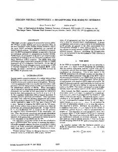
Fig. 2. The thick solid line represents the instantaneous frequency given by the polynomial in (14) and the dashed line represents the instantaneous frequency of a linear frequency modulated signal.
The task of designing the phase spectrum with the appropriate instantaneous frequency function still remains. In this paper, the desired phase spectrum is given by ! # $ %&" φd (f ) = arg F w(n) sin 2πθ(n/fs ) , (12)
where t = n/fs . The function w(n) was chosen as a Tukey window with 10% tapering. The phase in (12) is given by ' t fi (τ )dτ, T ≥ t ≥ 0, (13) θ(t) = 0
where fi (t) is the instantaneous frequency and is approximated by a third order polynomial (solid curve in Fig. 2) fi (t) = at3 + bt2 + ct + d, 0 ≤ t ≤ T
where the matched filtered spectrum would be D(f )D∗ (f ) = Ad (f )ejφd (f ) Ad (f )e−jφd (f ) = |Ad (f )|2 . (11) The axial response will therefore only depend on the inverse Fourier transform of the amplitude spectrum squared. To obtain an axial response with a low range sidelobe level, it is essential to choose a spectral shape which inverse Fourier transform has a low sidelobe structure. In this paper the Kaiser window will be used [9].
11
4
SIGNALS
,
6
9
III. D ESIGNING NON LINEAR FREQUENCY MODULATED
D(f ) = Ad (f )e
5
Instantaneous frequency
where I is the identity matrix, so that (7) simplifies to 1 H ˆs = W D. (9) M The result in (9) is equivalent to the N first samples of the inverse Fourier transform of the discrete spectrum D.
jφd (f )
4
10
(8)
A. Designing the amplitude spectrum If a matched filter is used as a compression operator, the phase of the transmitted waveform will be completely canceled. The phase will therefore not influence the axial response after pulse compression. The shape of the axial response will instead solely be determined by the squared amplitude spectrum of the transmitted waveform. However, the phase of the spectrum will influence the amplitude of the transmitted waveform. Since ultrasound systems are amplitude limited (due to the maximum excitation voltage of the transmitters) it is crucial to keep the amplitude of the waveform as close to the full excitation voltage as possible during the entire waveform. To illustrate this, consider again the desired spectrum of the excitation waveform
3
Fig. 1. The desired amplitude spectrum represented as the gray curve and the obtained amplitude spectrum when using the solid curve in Fig. 2 as instantaneous frequency is given as the black curve.
where W H is the complex conjugate transpose of W. Furthermore, the column vectors of W will be orthonormal as long as M ≥ N . A unique solution to (6) will therefore always exist as long as this condition is fulfilled. Moreover, if M ≥ N , the orthonormal property of the column vectors of W results in W H W = M I,
Desired Obtained
0
(14)
where the coefficients {a, b, c, d} are given in Table I when time is given in µs. The coefficients are chosen to enforce a constant amplitude level on the central part of the wave. The design method, step by step can be summarized as • Choose the desired amplitude spectrum Ad (f ). • Choose an appropriate polynomial to approximate the instantaneous frequency function fi (t). • Integrate fi (t) according to (13).
1715
2006 IEEE Ultrasonics Symposium
Coeff. a b c d
Value 0.0013 -0.0391 0.5104 3.5000
created by focusing 16 adjacent transducer elements 5 mm behind the face of the transducer generating a transmitting aperture with an F-number of 1.5. In total 112 transmissions were carried out before a complete image could be formed. In all phantom experiments, a Hanning apodization was used in receive over the 128 emulated receiving elements. In the in-vivo experiments, the active receiving aperture was 64 transducer elements, which acted as a sliding aperture and was centered around the active virtual source in that transmission.
TABLE I C OEFFICIENTS FOR THE POLYNOMIAL APPROXIMATING THE INSTANTANEOUS FREQUENCY CURVE
• • •
Sample θ(t) and calculate φd (f ) according to (12). Calculate D(f ) according to (10). Calculate the waveform using (9).
C. Reference experimental setup In the reference experiment a linear frequency modulated signal was used. This signal has previously been suggested and implemented successfully in STA systems for clinical trials [13]. The duration of the waveform was 20 µs, the bandwidth was 7 MHz and the center frequency was 7 MHz. A Tukey window with 10% tapering was applied on the transmitted waveform to reduce ripples in the passband of the amplitude spectrum. The use of mismatched filtering has been suggested to reduce temporal sidelobes [4], and the compression filter was therefore the time reversed excitation waveform with a Chebyshev-window applied. The relative sidelobe attenuation applied on the Chebyshev-window was 70 dB.
Waveform NLFM, polynomial approx. 1
Amplitude
0.5
0
−0.5
−1
0
2
4
6
8
10 Time µs
12
14
16
18
Fig. 3. The obtained waveform with center frequency 6 MHz, bandwidth 5 MHz, duration 20 µs, when using the instantaneous frequency given in Fig. 2.
D. Non-linear waveform experimental setup The waveform designed in Fig. 3 was used as the excitation waveform, and the time reversed version provided a compression filter. The energy of the proposed non-linear FM signal was 71% of the energy of the reference waveform.
Corr. receiver NLFM 0
Amplitude
−20
−40
E. Tissue mimicking phantom experiments
−60
−80
−100
−15
−10
−5
0 Time µs
5
10
15
Fig. 4. The envelope of the auto-correlation of the waveform for the polynomial approximation to the instantaneous frequency function. The axial sidelobes are approximately at -80 dB compared with the mainlobe.
IV. E XPERIMENTS A. Experimental equipment For the experimental part of this investigation the research scanner RASMUS [10] was used together with a BK8804 linear array transducer. The acquired data are stored in the system and can be extracted for offline processing on a Linux cluster. B. Data acquisition process In this paper a synthetic transmit aperture imaging technique was used [11]. In each transmission a virtual source [12] was
The next experiment was carried out on a tissue mimicking phantom from Dansk Fantom Service (Jyllinge, Denmark) to evaluate penetration depth. The attenuation in the phantom is 0.5 dB/[cm MHz] at 20◦ C. Inside the phantom metal wires are suspended, so that penetration depth can be evaluated. The results are given in Fig. 5 with 40 dB dynamic range. The penetration depth for the linear FM signal is approximately 10 cm, whereas the penetration depth for the non-linear FM signal was 11 cm. This is an increase of 1 cm and corresponds to an increase in SNR of 7 dB at a center frequency of 7 MHz. The measured gain in SNR is shown as the solid curve in Fig. 6 together with the expected gain as the gray dashed curve.
F. In-vivo experiments The carotid artery of a 27 year old healthy male was scanned. The signals were match filtered, beamformed, envelope detected and displayed using a dynamic range of 45 dB. The resulting images can be seen in Fig. 7, where the top image represents the linear FM experiment, and the bottom image shows the result for the non-linear FM experiment.
1716
2006 IEEE Ultrasonics Symposium
STA LFM
10
STA NLFM 20
30
30
40
40
Measured Theoretical
8 Gain SNR dB
20
6
4
50
50
60
60
70
70
80
80
90
90
100
100
110
110
120
120
0
20
30
40
50 Depth mm
60
70
80
Fig. 6. The theoretic gain in SNR as the gray dashed curve. The predicted gain was 4.9 dB. The measured gain as a function of depth is given as the black solid curve. STA NLFM
STA LFM
Axial position [mm]
Axial position [mm]
2
15
15
20
20
25
25
30
30
35
35
−10
130 130 −10 0 10 −10 0 10 Lateral position [mm] Lateral position [mm]
0 10 Lateral position [mm]
−10
0 10 Lateral position [mm]
Fig. 7. The common carotid artery of a 27 year old healthy male volunteer. The left image displays the reference experiment whereas the right image displays the proposed waveform. The dynamic range in both images is 45 dB.
Fig. 5. The experimental results for the tissue mimicking phantom. The attenuation is 0.5 dB/[cm MHz]. The result for the linear FM signal can be seen in the left image and the result for the proposed non-linear FM signal can be seen in the right image. The non-linear FM signal exhibits approximately 1 cm better penetration depth. At 7 MHz this corresponds to an increase in SNR of ≈7 dB.
V. C ONCLUSION A method for designing waveforms with attractive spectral properties has been presented. The method was used to design a waveform with temporal sidelobes at -80 dB compared to the mainlobe. The method has been tested and compared experimentally to a linear FM signal with the same duration. Even-though the non-linear FM signal only had 71% of the energy compared to the reference excitation, an increase of 4.9 dB in SNR was measured. VI. ACKNOWLEDGMENT This work was supported by grant 274-05-0327 from the Danish Research Agency, the Radio-parts foundation and by B-K Medical A/S, Denmark. R EFERENCES [1] J. A. Jensen, Estimation of Blood Velocities Using Ultrasound: A Signal Processing Approach, Cambridge University Press, New York, 1996. [2] M.I. Skolnik, Introduction to Radar Systems, McGraw-Hill, New York, 1980. [3] M. O’Donnell, “Coded excitation system for improving the penetration of real-time phased-array imaging systems,” IEEE Trans. Ultrason., Ferroelec., Freq. Contr., vol. 39, pp. 341–351, 1992.
[4] T. X. Misaridis and J. A. Jensen, “An effective coded excitation scheme based on a predistorted FM signal and an optimized digital filter,” in Proc. IEEE Ultrason. Symp., 1999, vol. 2, pp. 1589–1593. [5] FDA, “Information for manufacturers seeking marketing clearance of diagnostic ultrasound systems and transducers,” Tech. Rep., Center for Devices and Radiological Health, United States Food and Drug Administration, 1997. [6] R. E. Millett, “A matched-filter pulse-compression system using nonlinear fm waveform,” IEEE Trans. Aerosp. Elect. Syst., vol. 6, pp. 73–78, 1970. [7] M. Pollakowski and H. Ermert, “Chirp signal matching and signal power optimization in pulse-echo mode ultrasonic nondestructive testing,” IEEE Trans. Ultrason., Ferroelec., Freq. Contr., vol. 41, pp. 655–659, 1994. [8] L. Ljung, System Identification, theory for the user, Prentice-Hall., New Jersey, 1987. [9] D. H. Johnson and D. E. Dudgeon, Array signal processing. Concepts and techniques., Prentice-Hall., Englewood Cliffs, New Jersey, 1993. [10] J. A. Jensen, O. Holm, L. J. Jensen, H. Bendsen, S. I. Nikolov, B. G. Tomov, P. Munk, M. Hansen, K. Salomonsen, J. Hansen, K. Gormsen, H. M. Pedersen, and K. L. Gammelmark, “Ultrasound research scanner for real-time synthetic aperture image acquisition,” IEEE Trans. Ultrason., Ferroelec., Freq. Contr., vol. 52 (5), May 2005. [11] S. I. Nikolov, Synthetic aperture tissue and flow ultrasound imaging, Ph.D. thesis, Ørsted•DTU, Technical University of Denmark, 2800, Lyngby, Denmark, 2001. [12] M. O’Donnell and L. J. Thomas, “Efficient synthetic aperture imaging from a circular aperture with possible application to catheter-based imaging,” IEEE Trans. Ultrason., Ferroelec., Freq. Contr., vol. 39, pp. 366–380, 1992. [13] M. H. Pedersen, K. L. Gammelmark, and J. A. Jensen, “In-vivo evaluation of convex array synthetic aperture imaging,” Ultrasound Med. Biol., p. Submitted, 2004.
1717
2006 IEEE Ultrasonics Symposium