We describe an iterative multilevel method for solving linear systems representing forward modeling and back propagation of wavefields in frequency-domain ...
An iterative multilevel method for computing wavefields in frequency-domain seismic inversion Yogi A. Erlangga∗ and Felix J. Herrmann SUMMARY We describe an iterative multilevel method for solving linear systems representing forward modeling and back propagation of wavefields in frequency-domain seismic inversions. The workhorse of the method is the so-called multilevel Krylov method, applied to a multigrid-preconditioned linear system, and is called multilevel Krylov-multigrid (MKMG) method. Numerical experiments are presented for 2D Marmousi synthetic model for a range of frequencies. The convergence of the method is fast, and depends only mildly on frequency. The method can be considered as the first viable alternative to LU factorization, which is practically prohibitive for 3D seismic inversions. INTRODUCTION Imaging of the earth’s subsurface can computationally be done in the frequency domain by inverting seismic data using the adjoint-state method; see, e.g., Plessix (2006). One advantage, among others, of doing inversion in the frequency domain is the possibility of inversion with only a small subset of random frequencies, as shown, e.g., in Sirgue and Pratt (2004) and Mulder and Plessix (2004). In relation to this, it is demonstrated by Lin et al. (2008) (in this proceedings) that it is possible to recover the wavefield with only 30 per cent of frequencies required by the classical Nyquist sampling theory, by solving a sparsity-promoting recovery problem in, e.g., the Fourier domain. In combination with less number of grid points required to resolve the wavefield, seismic inversion in the frequency domain will now require less complexity as compared to the time domain migration. Translated to the seismic language, the adjoint-state method consists of forward modeling, in which a wave equation is solved for a given velocity background and source position, and computing a correction to the given velocity background. The correction is determined by minimizing the misfit between the seismic data, recorded at the receiver positions, and the forward model data at the positions corresponding to the physical receivers. The gradient of the misfit functional is closely related to the migrated image in geophysical applications, and can be computed by multiplication of forward and back propagated wavefields. These wavefields are computed via a finitedifference approximation of the wave equation.
three dimensions, work and storage needed by an LU factorization becomes O(n3x n3y n3z ) and 2n2x n2y nz , respectively. Considering these facts, it is considered prohibitively expensive to do frequency-domain seismic inversion based on LU factorization. Iterative methods are usually considered as an alternative to direct methods (Saad (2003)). An iterative method relies mostly on matrix-vector multiplications with A. Hence, an iterative method is less demanding in terms of memory and computational complexity. Iterative methods are, however, generally less robust as compared to direct methods, and in particular for wave simulations, all efficient, ad hoc iterative methods fail to converge for frequency as high as 5 Hz, in the case of, e.g., the 2D Marmousi synthetic model. Erlangga et al. (2006) proposed an iterative method based on Krylov subspace method, preconditioned by a damped acoustic wave operator. The preconditioner is inverted approximately by one multigrid iteration. In this paper, we call this method the MG method. While the method improves the convergence significantly, the convergence still shows dependence on angular frequency. In this paper, we will show that the convergence can be further improved if the MG method is used within the context of the multilevel Krylov method, called the MK method, recently introduced in Erlangga and Nabben (2007). We call this combination “the MKMG method”. THEORY For frequency-domain seismic imaging, the wavefield can be modeled by the frequency-domain acoustic wave equation „ « ω2 H u(ω, xs ; x) := − ∇ · ∇ − u(ω, xs ; x) = b, (1) c(x)2 equipped with radiation boundary conditions, where ω = 2π f , with f the frequency in Hz, and shot position xs .Application of finite differences on Equation 1 results in the linear system A[c]s us = bs ,
A ∈ Cn×n ,
(2)
As mentioned, e.g., in Pratt et al. (1998), wavefield computations may be done by direct methods, by first constructing the LU factors of the finite-difference wave equation matrix A. Once these factors are available, for a given angular frequency ω and velocity background c(x), both forward modeling and back propagation problems can be solved using the same LU factors for a set of shot-receiver positions.
where the vector u is a discrete approximate solution to the solution function u evaluated on the finite-difference grid points. In seismic inversions, we are concerned with the (real) velocity background associated with the wavefield data recorded at the receiver positions. Given a reasonable initial velocity background c and the corresponding solution vector u of the forward model 2, the real velocity background can be estimated by minimizing the functional F = 21 hδ d, δ di, where δ d := u(ω, xs ; xr ) − d(ω, xs ; xr ) defines the misfit between the forward model wavefield at the receiver positions, u(ω, xs ; xr ), and the seismic data d(ω, xs ; xr ). This minimization amounts to an update c`+1 = c` − α∇c F, (3)
Computing the LU factor of A is, however, very costly and memory consuming. In two dimensions, for example, computing LU factors require O(n2x nz ) work and ∼ 2n2x nz storage. In
where ∇c F = real{JH δ d}, and J = J(u, c) the Jacobian matrix of u with respect to c. Computing the Jacobian matrix is very costly, and in practice, only the action of the Jacobian on δ d is
Multilevel method in seismic inversion
(4)
∇c F =
(5)
By virtue of Equation 5, a frequency-domain seismic imaging now amounts to computing forward and back-propagated wavefields from Equations 2 and 4, respectively. In the next section, we describe an iterative method used to perform these computations. Methods The main driver for our method is the Krylov subspace method. It is well known that the convergence of a Krylov method depends to some extend on the eigenspectrum of the given matrix. In particular, if the condition number of A, denoted by κ(A), is small (or more specific, close to one), then the convergence of a Krylov method can be expected to be fast. For Equations 2 and 4, κ(A) is typically very large, called illconditioned. In order to have a better conditioning, an equivalent, right preconditioned system is solved, namely ˆ u = M−1 u,
(6)
where M is a preconditioning matrix. Note that we have dropped the superscript s to simplify the notation. For some class of matrices, the matrix M−1 is usually formed as a sort of approximation to A−1 . But, following Erlangga et al. (2006), M can be based on a finite-difference approximation of the damped, or shifted, wave operator ω2 (1 − β i), c(x)2
10
0.5
* 0 *********************
−20 0
1
2
i=
√ −1,
(7)
with β > 0. In this case, the matrix M is not an approximation of A in the usual sense. But, considering the preconditioned Equation 6, the matrix AM−1 has the following spectral properties. First, the eigenvalues of AM−1 are enclosed by a circle with center along the real axis of the complex plane. The center and the radius of the circle depends on the choice of β , but this circle never touches lines real = 0 and real = 1. This is sketched in Figure 1 (b). Hence, compared to the eigenspectrum of A, shown in Figure 1 (a), the eigenspectrum of AM−1 is very much clustered. Furthermore, while the real part of eigenvalues of A changes sign (called indefinite), the real part of eigenvalues of AM−1 all have the same sign. For a given β , the enclosing circle is independent of the finite-difference grid size h and angular frequency ω. Secondly, the largest eigenvalue of AM−1 in magnitude is bounded above by one. Thirdly, the smallest eigenvalue lies very close to zero at a
***** **** ** **** *** *******
0
−1.0 −0.5
3 10 4
(c) 1.0
−0.5
real( λ)
where UH = [u1 . . . uS ] and VH = [v1 . . . vS ]. The term ∇c F therefore corresponds to the migrated image in seismic imaging.
M := −∇ · ∇ −
(b) 1.0
−10
ω2 diag(UH V), c3
AM−1 uˆ = b,
imag( λ)
with (As )H the adjoint of As in Equation 2. For a set of shots s = 1, . . . , S, the gradient can be written as
(a) 20
imag( λ)
(As )H vs = δ ds ,
distance O(ω −1 ). The first two spectral properties guarantee h-independent convergence, and by the last property we may expect convergence mildly dependent of ω.
imag( λ)
needed. This is equivalent to back-propagating waves from the receiver positions. In this case, the back-propagated wavefield vs is computed from
0
0.5
1.0
0.5 0
****
−0.5
1.5
−1.0 −0.5
real( λ)
0
0.5
1.0
1.5
real( λ)
Figure 1: Illustration of the spectrum of (a) A, (b) AM−1 , and (c) AM−1 Q. The asterisks “ ” show the eigenvalues. It is worth noting that in practice M−1 is never computed exactly. Rather, in preconditioning steps in a Krylov subspace method, the action of M−1 on a vector is done approximately by one multigrid iteration. In this case, the preconditioning steps can be carried out with only O(nx nz ) work in 2D and O(nx ny nz ) work in 3D. Details of this technique are discussed in Erlangga et al. (2006) and Riyanti et al. (2006a), where BiCGSTAB (van der Vorst (1992)) is used for the Krylov iteration. Throughout the paper, Bi-CGSTAB preconditioned by multigrid will be in short referred to as the MG method. As the largest eigenvalue is always bounded above by one, it appears that the convergence of the MG method is now solely determined by the small eigenvalues of AM−1 , which is of order ω −1 . Hence, convergence can be further improved if these small eigenvalues are somehow shifted to some values far from zero. This shift should however be performed such that the upper bound of the eigenspectrum remains the same. Such a “spectral modification” is done by the so-called multilevel Krylov (MK) method, introduced recently by Erlangga and Nabben (2008) and Erlangga and Nabben (2007). Define a projection Q as Q := I − ZE−1 YT AM−1 + λn ZE−1 YT ,
(8)
with E := YT AM−1 Z ∈ Cm×m , λn the largest eigenvalue of AM−1 in magnitude, and Z, Y ∈ Rn×m , m � n, any rank m projection matrices. In this case, n = nx nz in 2D, or n = nx ny nz in 3D. A convergence acceleration of a Krylov method is obtained if it is applied to the system AM−1 Qu˜ = b,
˜ u = M−1 Qu.
(9)
The effect of the inclusion of Q can be briefly explained as follows. Denote the eigenspectrum of AM−1 by σ (AM−1 ) = {λ1 , . . . , λn } ∈ C,
(10)
where λ ’s are ordered such that |λ1 | ≤ |λ2 | · · · ≤ |λn |. In this case, |λn | → 1, and |λ1 | = O(ω −1 ). For any full rank Z, Y, the eigenspectrum of AM−1 Q becomes σ (AM−1 Q) = {µ1 , . . . , µn } ∈ C.
(11)
Because |λn | → 1, in this case |µn | → 1 and |µi | = O(λn ) = O(1). This is illustrated in Figure 1 (c), which shows that the eigenvalues of AM−1 are now moved towards 1, due to the
Multilevel method in seismic inversion
A brief discussion on the implementation aspects of the MKMG method is given in Appendix A. For more details, see Erlangga and Nabben (2008) and Erlangga and Nabben (2007).
0 200 400 depth (m)
inclusion Q. Since µi now is O(1), the condition number of AM−1 Q can be expected to be O(1). In terms of number of iterations, this will lead to a much faster convergence. The application of a Krylov method on Equation 9 results in the multilevel Krylov-multigrid method, or MKMG.
600 800 1000 1200 1400
EXAMPLE AND DISCUSSION Numerical experiments are performed based on a part of 2D Marmousi synthetic model as shown in Figure 2. We consider two situations encountered in frequency-domain inversions: forward and back-propagation model, governed by Equations 2 and 4, respectively. To mimic forward modeling, a point source is located at the position (3000, 50) m. For back propagation, we consider point sources distributed along the receiver line at z = 50 m. In both cases, f = [5, 30] Hz is used.
1600 0
1000
2000
3000 4000 x−axis (m)
5000
6000
Figure 3: Wavefield from forward modeling. f = 20 Hz. 300 MKMG 250
MG
200 150
0
100
200
50
depth (m)
400
0 0
5
600 800
10 15 20 Frequency, Hz
25
30
Figure 4: Forward modeling using 2D Marmousi velocity model. Black lines indicate the number of iterations; the gray lines are the number of multiplications with A.
1000 1200 1400 1600 0
1000
2000
3000 4000 x−axis (m)
5000
6000
Figure 2: Part of 2D Marmousi data. cmin = 1500 m/s, cmax = 4450 m/s. As aforementioned, in the MG method, Bi-CGSTAB is applied on Equation 6. For MKMG, we apply GMRES (Saad and Schultz (1986)) on Equation 9. In this case, both methods require two matrix-vector multiplications with A and two preconditioner solves by one multigrid iteration per iteration; thus, they amount to approximately the same complexity. We set Y = Z, with Z associated with the bilinear interpolation of the coarse grid into the fine grid. The iteration is terminated if the initial residual has been reduced by six orders of magnitude. A snapshot of forward modeling at f = 20 Hz is shown in Figure 3. We note that it is theoretically difficult to determine the optimal β in Equation 7 for MKMG. In this case, we have to rely on numerical experiments. We found that β = 1 is the best value we could obtain so far. This value of β is different from the MG method, where β = 0.5. Convergence results of MKMG for forward and back-propagation problems are shown in Figure 4 and Table 1, respectively, with 1 the grid size h ≈ 18 cmin / f . The results indicate that there is practically no significant difference in convergence for forward and back-propagation problems. With β = 1, the convergence of MKMG is practically independent of frequency.
In Figure 4, we also compare the convergence results of MKMG with the MG method. In terms of the number of iterations, MKMG converges about five times faster than the MG method. It is worth mentioning that without any preconditioner, BiCGSTAB applied to Equation 2 with f = 1 Hz requires 17446 iterations to converge. Table 2 compares the convergence results of MKMG in Figure 4 with the case where the grid size is fixed. In this case, 1 for f = [5, 30] Hz we set h = 18 (cmin /30). Hence, for low frequencies the grid used is extremely fine. The table clearly shows that the convergence is independent of h. Frequency (Hz)
5
10
15
20
25
30
Iteration count
8
10
11
15
15
23
Table 1: Number of MKMG iterations for back propagation using 2D Marmousi velocity model. Finally, we estimate the total memory used in MKMG and compare it with direct methods in the case of in-core implementation. (MKMG can however be implemented without any matrices stored in memory.) For MKMG, we need to store the matrices A’s, M’s, and Z’s (see Appendix A). In addition, since we base the MKMG method on GMRES, we also need to store vectors of length nx nz used in GMRES. As seen in Figure 5, MKMG requires less memory than LU factorization.
Multilevel method in seismic inversion Frequency (Hz)
5
10
15
20
25
30
APPENDIX A
Grid adapted to f
8
10
11
15
15
23
THE MKMG METHOD
Grid fixed at f = 30 Hz
8
8
11
12
15
23
To describe the MKMG method, we rewrite Equation 9 as
Table 2: Number of MKMG iterations for forward modeling using the 2D Marmousi data.
This advantage will become more significant in three dimensions. 10
10
LU MKMG 9
Unit memory
10
8
˜ = b, A1 M−1 1 Q1 u
˜ u = M−1 1 Q1 u,
(A-1)
−1 −1 T T with Q1 := I1 −Z12 E−1 2 Y12 A1 M1 +λn Z12 E2 Y12 , and E2 := −1 T Y12 A1 M1 Z12 . Note that the matrix Q1 must not be constructed explicitly because Q1 is dense. The reason of choosing of subscripts in this manner will be clear during the discussion. Suppose that we have Y12 and Z12 .
In a Krylov method, the solution subspace is expanded by computing the new basis wi+1 using the previous basis wi , i.e., “ ” i −1 T i ˆ ,(A-2) wi+1 = A1 M−1 wi − Z12 E−1 1 Q1 w = A1 M1 2 Y12 w
10
7
10
6
10
10
15
20 Frequency, Hz
25
30
Figure 5: Memory used in LU factorizations and MKMG. CONCLUDING REMARKS Parallel implementations of the MG method have been presented for 2D and 3D forward modeling in Kononov et al. (2006) and Riyanti et al. (2006b), respectively. Since Krylov methods are well parallelizable, this implies that the MKMG method is also well parallelizable. Riyanti et al. (2006b) note that the 2D frequency-domain migration based on direct methods can be about one order of magnitude faster than the 2D time-domain migration. For direct methods with nested dissection, computing LU factors and linear system solves amount to n f O(n3 ) = n f nO(n2 ) and n f ns O(n2 log n) work, respectively, with n f the number of frequencies, ns the number of shots, and n = nx = nz . Thus, if ns = n, the complexity is WD = n f ns (O(n2 ) + O(n2 log n)). In direct methods, however, the equality constant for the first term is usually large. For MKMG, the complexity is WMKMG = n f ns nit O(n2 ), with nit the number of MKMG iterations. Since for n > e, n2 log n > n2 , we see that WMKMG < Cn f ns n2 log n if the corresponding equality constant times nit is smaller than C log n. Considering its fast convergence, it is very likely that for 2D problems, MKMG is more efficient than the most efficient direct methods. This efficiency of MKMG will be more pronounced in 3D. Combining MKMG with sparsity-promoting recovery, which allows the use of a very limited number of frequencies, will further widen the margin between the frequencydomain and time-domain migration. ACKNOWLEDGMENTS This work was in part financially supported by the NSERC Discovery (22R81254) and CRD Grants DNOISE (33481005) and was carried out as part of the SINBAD project with support, secured through ITF, from BG Group, BP, Chevron, ExxonMobil and Shell.
i ˆ i = (A1 M−1 ˆ := YT12 w ˆ i , with yˆ ∈ where w 1 − λn I1 )w . Define y −1 m C . We then need to compute zˆ = E2 yˆ . We avoid an explicit computation of E−1 because we need to form M−1 1 , which, in our case, is not available because we only know the action of it on a vector via one multigrid iteration. Rather, we will only consider the action of E−1 on yˆ via the implicit equation
E2 zˆ = yˆ .
(A-3)
To do this, we introduce an approximation to E2 of the form E2 ≈ YT12 A1 Z12 (YT12 M1 Z12 )−1 YT12 Z12 .
(A-4)
The products YT12 A1 Z12 =: A2 , YT12 M1 Z12 =: M2 and YT12 Z12 =: B2 are the Galerkin approximation associated with the individual matrices A1 , M1 , and B1 = I1 , respectively, and have a very similar form with the coarse-grid matrix in multigrid. Hence, the matrices Y12 and Z12 can be built in the same way the multigrid interpolation and restriction matrix. Since m = dimA2 = dimM2 = dimB2 � dimA1 = n, we say that the ˆ and respectively zˆ , belong to a higher and lower divectors w, mension subspace. All matrices which map a vector into the largest subspace are denoted by the subscript “1”, etc. To get an accurate zˆ as fast as possible, we can introduce an operator Q2 , which is similar to Q1 . By virtue of approximation A-4, zˆ is solved from Equation A-3 by solving the system ˆ, A2 M−1 2 B2 Q2 z˜ = y
zˆ = Q2 z˜ .
(A-5)
By an application of a Krylov method on Equation A-5, a recursive MKMG method results. An MKMG method with four levels is illustrated in Figure A-1. Level 1 : A Level 2 : E Level 3 : E3 Level 4 : E4
Figure A-1: One MKMG iteration. Black circles indicate the MK step, the white circles indicate the MG loop.
Multilevel method in seismic inversion REFERENCES Erlangga, Y. A. and R. Nabben, 2007, On multilevel projection krylov method for the preconditioned helmholtz system: Electronic Transaction in Numerical Analysis, submitted. ——–, 2008, Multilevel projection-based nested Krylov iteration for boundary value problems: SIAM Journal on Scientific Computing, to appear. Erlangga, Y. A., C. W. Oosterlee, and C. Vuik, 2006, A novel multigrid-based preconditioner for the heterogeneous Helmholtz equation: SIAM Journal on Scientific Computing, 27, 1471–1492. Kononov, A. V., C. D. Riyanti, S. W. de Leeuw, C. Vuik, and C. W. Oosterlee, 2006, Numerical performance of parallel solution of heterogeneous 2d Helmholtz equation: Computing and Visualization in Science, online http://www.springerlink.com/content/6q377635t271624m/. Lin, T. T. Y., E. Lebed, Y. A. Erlangga, and F. J. Herrmann, 2008, Interpolating solutions of the Helmholtz equation with compressed sensing: Presented at the SEG Meeting, this proceedings. Mulder, W. A. and R. E. Plessix, 2004, How to choose a subset of frequencies in frequency-domain finite-difference migration: Geophysical Journal International, 158, 801–812. Plessix, R. E., 2006, A review of the adjoint-state method for computing the gradient of a functional with geophysical applciations: Geophysical Journal International, 167, 495– 503. Pratt, R. G., C. Shin, and G. J. Hicks, 1998, Gauss-Newton and full Newton methods in frequency-space seismic waveform inversion: Geophysical Journal International, 133, 341– 362. Riyanti, C. D., Y. A. Erlangga, R. E. Plessix, W. A. Mulder, C. Vuik, and C. W. Oosterlee, 2006a, A new iterative solver for the time-harmonic wave equation applied to seismic problems: Geophysics, 71, E57–E63. Riyanti, C. D., A. Kononov, Y. A. Erlangga, C. Vuik, C. W. Oosterlee, R. E. Plessix, and W. A. Mulder, 2006b, A parallel multigrid-based preconditioner for the 3d heterogeneous high-frequency Helmholtz equation: Journal of Computational Physics, 224 (1), 431–448. Saad, Y., 2003, Iterative methods for sparse linear systems: SIAM. Saad, Y. and M. H. Schultz, 1986, GMRES: A generalized minimal residual algorithm for solving nonsymmetric linear systems: SIAM Journal on Scientific Computing, 7(12), 856–869. Sirgue, L. and R. G. Pratt, 2004, Efficient waveform inversion and imaging: A strategy for selecting temporal frequencies: Geophysics, 69, 231–248. van der Vorst, H. A., 1992, Bi-CGSTAB: a fast and smoothly converging variant of BI-CG for the solution of nonsymmetric linear systems: SIAM Journal on Scientific Computing, 13(2), 631–644.