At the same time, the benefits of sparsity for single channel deconvolution problems .... with a practical learning step on A to complete the algorithm. IV. KNOWN ...
1
An iterative thresholding algorithm for joint deconvolution and separation of multichannel data Y. Moudden, J. Bobin and J.-L. Starck CEA, IRFU, SEDI, Centre de Saclay, F-91191 Gif-sur-Yvette, France
Abstract—We report here on extending GMCA to the case of convolutive mixtures. GMCA is a recent source separation algorithm which takes advantage of the highly sparse representation of structured data in large overcomplete dictionaries to separate components in multichannel data based on their morphology. Many successful applications of GMCA to multichannel data processing have been reported : blind source separation, data restoration, color image denoising and inpainting, etc. However, the data model in GMCA assumes an ideal instrument, not accounting for instrumental impulse response functions which can be crucial in some important applications such as CMB data analysis from the Planck experiment. We show here how to build on GMCA for that purpose and describe an iterative thresholding algorithm for joint multichannel deconvolution and component separation. Preliminary numerical experiments give encouraging results. Index Terms—Multichannel data, Blind source separation, multichannel deconvolution, overcomplete representations, sparsity, morphological component analysis, GMCA, morphological diversity.
I. I NTRODUCTION In preparation for the challenging task of analyzing the fullsky CMB maps that will shortly be available from ESA’s Planck1 experiment, dedicated multichannel data processing methods are being actively developed. A precise analysis of the data is of huge scientific importance as most cosmological parameters in current models are constrained by the statistics (e.g. spatial power spectrum, Gaussianity) of the observed primordial CMB field [1]. A first concern is that several distinct astrophysical processes contribute to the total observed radiation in the frequency range used for CMB observations [2]. The task of unmixing the CMB, the Galactic dust and synchrotron emissions, the contribution of the Sunyaev-Zel’dovich (SZ) effect of galaxy clusters, to name a few, has attracted much attention. Several generic and dedicated source separation algorithms have been applied and tailored to account for the specific prior knowledge of the physics at play ( [3]–[5] and references therein). Among these methods, GMCA (Generalized Morphological Component Analysis) has proven to be an efficient and flexible source separation algorithm. GMCA takes advantage of the sparse representation of structured data in large overcomplete signal dictionaries to separate sources based on their morphology. A full description of GMCA is given in [6], [7] and its application to CMB data analysis is reported in [5]. 1 http://astro.estec.esa.nl/Planck
However, another issue is multichannel deconvolution : the different channels of practical instruments have different point spread functions. Hence, a correct fusion of the multichannel observations for the purpose of estimating the different astrophysical component maps, requires a simultaneous inversion of the spectral mixing (i.e. each component contributes to each channel according to its emission law) and of the spatial mixing (i.e. convolution by the instruments psf in each channel). Our purpose here is to extend the GMCA framework and propose and algorithm that can achieve such a joint deconvolution and separation. The devised method relies on the a priori sparsity of the initial components in given overcomplete representations (e.g. Fourier, wavelets, curvelets). It is an iterative thresholding algorithm with a progressively decreasing threshold, leading to a salient-to-fine estimation process which has proven successful in related algorithms ( [8]–[10] and references therein). Results of numerical simulations with synthetic 1D and 2D data are presented, in the specific case where the mixing parameters are fully known a priori. These preliminary toy experiments motivate current efforts to extend the range of applications to the more difficult case of blind separation where the mixing matrix and possibly the beams are unknown. We are also working on applying the proposed method to multichannel CMB data. II. L INEAR MIXING AND CHANNEL - WISE CONVOLUTION The simplest model encountered in the field of component separation states that the observations are a noisy linear instantaneous mixture of the initial components. Such a model has, for instance, often been used to describe multichannel CMB observations : the total sky emission observed in pixel j with detector i sums the contributions of n components xji
=
n X
aki sjk + nji
(1)
k=1
where sjk is the emission template for the k th astrophysical process, herein referred to as a source or a component. The coefficient aki reflects the emission law of the k th source in the frequency band of the ith sensor, and nji stands for the noise contributions to the observations. When t observations are obtained from m detectors, this equation can be put in a more convenient vector-matrix form: X = AS + N
(2)
where X and N are m × t matrices, S is n × t, and A is the m × n mixing matrix. For simplicity, the noise is assumed
2
uncorrelated intra- and inter- channel, with variance σk2 in the k th channel. Commonly, the different channels of typical multichannel instruments do not have the same, what is more high resolution, impulse response or point spread function (psf ). The above model is then not capable of correctly rendering the observations : assuming the psf ’s are known, fitting that model to the observations is not making the most of the data and will not produce estimates of the component maps at the best possible resolution. A notable exception is when the multichannel observations offer multiple views of a single process in which case there is no separation to be performed and the analysis can be reduced from a multichannel to a single channel deconvolution problem without loss of statistical efficiency [11]. As mentioned above, our interest here is with analyzing multiple convolutive mixtures of multiple sources, when the different channels have different point spread functions : X = H(AS) + N
(3)
denoting H the multichannel convolution matrix-operator, acting on each channel separately. The data observed in channel i is xi = ai SHi + ni (4) where Hi is the t × t matrix of the convolution operator in this channel, xi , ai and ni are respectively the ith lines of X, A and N . In practice, both the sources S and their emission laws A may be unknown, a case referred to as blind, or only partly known. Although blind deconvolution would be an added excitement, we consider here that the instrumental psf ’s are fully known a priori. The purpose of source separation algorithms is then to invert the mixing process and provide estimates of the unknown parameters. This is most often an illposed problem, requiring additional prior information in order to be solved : one needs to know what in essence makes the sources different. For instance, they may have a priori disjoint supports in a given representation such as time and/or frequency leading to clustering or segmentation algorithms. In some cases, knowing a priori that the mixed sources are statistically independent processes will enable their recovery : this is the framework of Independent Component Analysis (ICA), a growing set of multichannel data analysis techniques, which have proven successful in a wide range of applications [12]. Indeed, although statistical independence is a strong assumption, it is in many cases physically plausible. ICA algorithms for blind component separation and mixing matrix estimation depend on the a priori model used for the probability distributions of the sources [12]–[15]. An especially important case is when the mixed sources are highly sparse, meaning that each source is only rarely active and mostly nearly zero. The independence assumption then ensures that the probability for two sources to be significant simultaneously is extremely low so that the sources may again be treated as having nearly disjoint supports. It is shown in [16] that first moving the data into a representation in
which the sources are sparse greatly enhances the quality of the separation. Working with combinations of several bases or with very redundant dictionaries such as the undecimated wavelet frames, ridgelets or curvelets [17] leads to even sparser representations : this is exploited by GMCA. Sparsity is now generally recognized as a valuable property for blind source separation. At the same time, the benefits of sparsity for single channel deconvolution problems in signal and image processing have been experimented in [18]–[20]. Hence, the joint multichannel deconvolution and source separation problem presumably has much to gain from sparse representations in large dictionaries, with a GMCA-like recovery process. Following the assumptions in GMCA which we are extending here to the case of convolutive mixtures, we assume that the source processes have sparse representations in a priori known dictionaries. For the sake of simplicity, we consider that the components all have a sparse representation in the same orthonormal basis Φ. Recent analyses in [21]–[23] give theoretical grounds for an extension to frames and redundant dictionaries. We also assume that the source processes are generated from sparse coefficient vectors αi sampled identically and independently from Laplacian distributions P (αi ) ∝ exp (−λi kαi k1 )
(5)
with inverse scale parameter λi , and si = αi Φ. The linear operator considered here, linear mixing followed by convolution in each channel, is somewhat cumbersome to handle : mixing acts on each column of S separately while convolution acts on the each line of AS separately. The full operator does not factorize very nicely. The order in which the mixing and the convolution matrices apply obviously matters. In the case where A and H are invertible, inverting the full operator consists in first applying the inverse of H and then the inverse of A. When additive noise corrupts the observed data, or when the channel-wise convolution operator or the mixing matrix are underdetermined, inversion asks for some sort of regularization. We consider here inverting the joint mixture and convolution operator in a possibly underdetermined and noisy context thanks to regularization induced by the a priori sparsity of the component signals to be recovered. Making the most of the noisy data to estimate the sources neither reduces to applying the inverse of A and deconvolving each source separately, nor deconvolving each channel separately and applying the inverse of A. This is also true of estimating A with S fixed. A global necessarily intricate multichannel data processing is necessary. III. F ULL OBJECTIVE FUNCTION With the assumptions in the previous section, the joint deconvolution and separation task is readily expressed as a minimization problem, in all respects equivalent to a maximum a posteriori estimation of A and S assuming an improper uniform prior on the entries of A : X 1 λi ksi Φt k1 (6) min kX − H( AS )k2Σ + A,S 2 i
3
where the subscript Σ reminds us of the noise covariance matrix, and Φt is the transpose of Φ. Equivalently, one has : X X 1 ai αi Φ )k2Σ + λi kαi k1 (7) min kX − H( A,{αi } 2 i i The above objective balances between a quadratic measure of fit and an `1 sparsity measure of the solution. The `1 is used here in place of the combinatorial `0 pseudo norm which is the obvious sparsity constraint, however much less conveniently handled [24]. Still, the above problem is non convex. Nevertheless, starting form an initial guess, a solution of reduced cost can be reached using and iterative block coordinate relaxation approach [25], [26], where the pairs ai , si (ith column of A, ith line of S) are updated one at a time. Assuming without much loss of generality that Φ is the identity matrix, we have, alternating over i, the following minimization problems : 1 min kRi − H( ai si )k2Σ + λi ksi k1 2
(8)
ai ,si
where Ri = X − H(
X
aj sj )
(9)
j6=i
Rewriting the quadratic matrix norm with an explicit sum over lines leads to : X 1 kRi,k − aik si Hk k2 + λi ksi k1 (10) min i 2σk2 a ,si k
where Ri,k is the k th line of Ri . Keeping si fixed, zeroing the gradient of the above with respect to aik leads to the following update rule : �−1 t aik = si Hk Hkt sti si Hk Ri,k (11) Conversely, keeping ai fixed, zeroing the gradient2 of the above with respect to si leads to : si =
X ai k
R H t − λi sign(si ) 2 i,k k
k
σk
!
X “ ai ”2 k
k
σk
to reach and stay stuck by the local minimum closest to the starting point. In the following, we focus on approximations for faster and more robust algorithms and propose a practical rule for updating the components S assuming the mixing matrix A is known and fixed. Future work will combine this with a practical learning step on A to complete the algorithm. IV. K NOWN MIXING MATRIX When A is known a priori, problem (6) reduces to a linear inverse problem with a sparsity constraint on the solution : X 1 λi ksi k1 (13) min kX − H( AS )k2Σ + S 2 i In the single channel case, deconvolution with an l1 penalty has been studied previously with a known mixing matrix [18]– [20]. More generally, solving linear inverse problems with sparse priors or l1 regularization has attracted much attention lately [27]–[30]. If the combined mixture and convolution linear operator is underdetermined, the above cost function is not strictly convex. This is where sparse decomposition methods have proven especially profitable. When the operator is overdetermined, the l1 sparsity constraint is a useful regularization when the data is corrupted by noise : the available budget will hopefully not be spent on representing small noise coefficients. Theoretical results have been established regarding the existence and uniqueness of a solution, and general algorithms have been proposed to solve some of these problems ( [31] and references therein). In principle, these methods apply to the problem at hand. Among these, we focus on iterative projected descent algorithms which have been proposed in [29], [30], [32], [33] for the inversion of underdetermined linear operators with sparsity constraints. Consider again updating each source si alternately, assuming all the other sources fixed. The minimization problem (13) can be rewritten as follows : min f1 (ai , si ) + λi f2 (si )
!−1 Hk Hkt
si
(12)
provided the rightmost term exists. Save for the sign function, this is the least squares solution to the multichannel deconvolution in the single-input multiple-output (SIMO) case. An important feature here is the effective beam used for the deconvolution : the effective beam may be invertible even if the individual beams are not. Following the discussion in [11] any robust 1D deconvolution algorithm could be applied to the 1D-projected data. Here, as hinted to by the sign function, robustness will come from shrinkage. However, equation (12) is not easily inverted and probably has no closed form solution owing to the coupling matrix on the right which would commonly not be diagonal. It would have to be solved numerically in an iterative scheme, in the general case. When this factor is diagonal (or approximately diagonal), the closed form solution is known as soft-thresholding. In all cases, the full set of update rules leads to a slow algorithm which is likely 2 We stick to loose definitions, knowing that rigorous statements can be made with no impact on the result.
(14)
where f1 (ai , si ) =
X 1 kRi,k − aik si Hk k2 2σk2 k
and
f2 (si ) = ksi k1 (15)
The gradient of f1 with respect to si assuming all the other parameters are fixed is given by : � ai �2 X ai g= − k2 Ri,k Hkt + k si Hk Hkt (16) σk σk k
The Hessian of f1 is given by : X � ai �2 k H= Hk Hkt σk
(17)
k
From here, several optimization schemes are possible all akin to a projected descent algorithm, the descent direction is given by the conjugate gradient. Typically, following recent developments in optimization [29], [30], [32], [33]: � −1 snew = ∆λi sold (18) i i − µgH where ∆λi is a soft or hard thresholding operator with
4
0.5
threshold λi and µ is the usual step size parameter. It follows that : X k
! Ri,k Hkt
0
! H −1
−0.5
(19)
Taking a single step of length µ = 1 at each iteration leads to the following update rule : s i = ∆λi @
X k
aik σk2
! Ri,k Hkt
X “ ai ”2 k
k
σk
20
40
60
80
100
120
0
20
40
60
80
100
120
0
20
40
60
80
100
120
0.4 0.2 0 −0.2
0
0
0.6
amplitude
(1 − µ)sold i +µ
= ∆ λi snew i
aik σk2
!−1 1 Hk Hkt
A
1
(20)
0.5 0 −0.5
S
new
“ “ ”” = ∆{λi } S old + µAt Ht X − H(AS)
−1
sample number 1
amplitude
0.5 0 −0.5 −1 0
20
40
60 80 sample number
100
120
20
40
60 80 sample number
100
120
1 0.5 amplitude
which is simply thresholding the linear least squares solution. The numerical experiments in the next section were conducted using this rule to update each source alternately and iteratively. Following a specific feature of MCA and GMCA-like algorithms, the threshold is initially set to a high enough value and is progressively decreased along iterations, leading to a robust salient to fine estimation process. The strategy by which the thresholds are progressively decreased along the iterations is an important issue discussed in [34]. As mentioned earlier, the computation of the inverse Hessian should be better behaved than inverting each single channel deconvolution operator separately [11]. Other similar projected descent iterations with proper preconditioning were also experimented with but did not lead to better results. The following projected Landweber iteration,
0 −0.5 −1 −1.5 0
(21)
where µ is a small enough step size and Ht is the adjoint of the channel-wise convolution operator, used in conjunction with a decreasing threshold, is slow but leads to very similar results. Without the decreasing threshold, the latter iteration was even slower to convergence and less robust in recovering the mixed sources. Other preconditioners could be used to lower the complexity of the iteration such as the inverse diagonal or block-diagonal of the Hessian [23], or to handle cases where the Hessian is badly conditioned. Using a different step length for each scale, in a projected Landweber iteration to solve a wavelet-regularized deconvolution is an interesting possibility discussed in [35]. Current work is also on other iterations involving the inverse or pseudo inverse of A. After the sources S have been estimated for a given mixing matrix A, the next step consists in updating the mixing matrix using a suitable learning step. Alternating source estimation steps and mixing matrix learning steps is current research to be reported shortly. V. N UMERICAL EXPERIMENTS In a first set of experiments, with multichannel 1D data, source signals of length t = 128 were generated as Bernoulli spike trains with parameter p. The spikes were given random amplitudes uniformly distributed between −1 and 1. Random mixing matrices and beams were used. The latter are positive with compact support. The beams and columns of the mixing matrix were normalized to unit l2 norm. Noise was added to the mixed and convolved sources, sampled from a normal distribution with 0.1 standard deviation. The experiments were repeated 500 times.
Fig. 1. top : Synthetic mixtures in the three channels used in this experiment. bottom : The two original sources are in green. The source signals recovered using the proposed algorithm appear in red. The results obtained using a simple pseudo-inverse of the linear mixture and convolution operator appear in light blue.
Figure 1 shows typical synthetic observation in three channels. The joint separation and deconvolution objective was approached using the proposed alternating iterative progressive thresholding scheme (20). The results were compared to those obtained using a multichannel Wiener filter and a simple pseudo-inverse of the full linear operator. Figure 2 display a comparison of these three methods in terms of false postives to true postives curves, as the final threshold is decreased. The impact of an increasing number of channels, or an increasing sparsity of the sources, or an increasing noise variance on the performance of these algorithms is shown to agree with what is expected. In all cases, the proposed iterative thresholding scheme performs much better than the other two filters. In a second set of experiments, with multichannel 2D data, three natural images shown on the left of figure 5 were used to generate six random mixtures. These were then degraded by 2D-convolution resulting in the blurred images shown on figure 4, using the Laplacian beams shown on figure 3. Applying the proposed algorithm in the curvelet domain, enables a good recovery of the input images from the multichannel data as shown on figure 5 where the separated and deconvolved images are on the right.
5
0.45 0.4 50
50
100
100
150
150
200
200
0.35
true positives
0.3 0.25 0.2 0.15 250
250 50
100
150
200
250
50
100
150
200
250
50
100
150
200
250
50
100
150
200
250
0.1 0.05 50
50
100
100
150
150
200
200
0 0
0.05
0.1
0.15
false positives 0.6
0.5
250
true positives
250 50
0.4
0.3
0.2
100
150
200
250
50
50
100
100
150
150
200
200
0.1
0 0
0.02
0.04
0.06
0.08 0.1 0.12 false positives
0.14
0.16
0.18
0.2
250
250 50
100
150
200
250
1
Fig. 4. Simulated observations consisting of blurred linear mixtures of three intial images shown on figure 5, in six channels with psf ’s shown on figure 3.
0.9 0.8
true positives
0.7 0.6 0.5 50
50
100
100
150
150
200
200
0.4 0.3 0.2 0.1 0 0
0.02
0.04
0.06
0.08
0.1 250
false positives
250 50
Fig. 2. Curves in red were obtained using the proposed alternate iterative and progressive thresholding scheme. The pseudo-inverse gives the results in dark blue while the Multichannel Wiener Filter gives those in light blue. top : Lowering the Bernoulli parameter p from 0.4 to 0.1 gives sparser source processes for which the proposed scheme clearly performs better. middle : The standard noise deviation is lowered from 0.1 to 0.05, 0.025, 0.001 with the expected impact on the algorithms performance. bottom : Increasing the number of channels from 2 to 3, 4, 6 also leads to better source estimation.
100
150
200
250
50
50
100
100
150
150
200
200
250
channel 2
0.4
0.8
0.3
0.6
0.2
0.4
0.1 0
122
128
134
140
channel 4
1
0
100
150
200
250
116
122
128
134
140
channel 5
0
116
50
50
122
128
134
128
134
140
0
100
150
200
250
100
100
150
150
200
200
50
100
150
200
250
140
0.5 250 50
122
50
channel 6
1
0.5
116
250
0.5
250
0
200
1
1
0.5
150
channel 3
0.2 116
100
250 50
channel 1
50
116
122
128
134
140
0
116
122
128
134
100
150
200
250
140
Fig. 3. The six Laplacian beams used to obtain the blurred image mixtures shown on figure 4, by 2D convolution.
Fig. 5. left : The three initial images. right : The three recovered images using the proposed joint deconvolution and separation algorithm in the curvelet representation.
6
VI. F UTURE WORK The preliminary results reported here have demonstrated the feasibility of a joint separation and deconvolution of multichannel data. We described an alternating progressive iterative thresholding algorithm to obtain a robust inverse of the mixing and convolution linear operator. Current work is with extending this method to the case where the mixing matrix is not known a priori, much in the line of GMCA for blind source separation. The idea is to alternate updates of S and A, i.e. sparse coding and dictionary learning steps, in a salientto-fine process with a threshold decreasing along iterations. An important application is CMB data analysis, which will benefit from the versatility of GMCA-like algorithms which can easily account for prior knowledge of the emission laws of the mixed components. Assuming unknown but parametric psf ’s is yet another exciting perspective. R EFERENCES [1] G.Jungman et al, “Cosmological parameter determination with microwave backgroung maps,” Phys. Rev. D, vol. 54, pp. 1332–1344, 1996. [2] R.Gispert R.Bouchet, “Foregrounds and cmb experiments: I. semianalytical estimates of contamination,” New Astronomy, vol. 4, no. 443, 1999. [3] Jacques Delabrouille, Jean-Franc¸ois Cardoso, and Guillaume Patanchon, “Multi–detector multi–component spectral matching and applications for CMB data analysis,” Monthly Notices of the Royal Astronomical Society, vol. 346, no. 4, pp. 1089–1102, Dec. 2003, to appear, also available as http://arXiv.org/abs/astro-ph/0211504. [4] Jacques Delabrouille and Jean-Franc¸ois Cardoso, Data Analysis in Cosmology, chapter Diffuse source separation in CMB observations, Lecture Notes in Physics. Springer, 2007, Editors: Vicent J. Martinez, Enn Saar, Enrique Martinez-Gonzalez, Maria Jesus Pons-Borderia. [5] J. Bobin, Y. Moudden, J.-L. Starck, M.J. Fadili, and N. Aghanim, “Sz and cmb reconstruction using gmca,” Statistical Methodology, vol. 5, no. 4, pp. 307–317, 2008. [6] J. Bobin, Y. Moudden, and J.-L. Starck, “Enhanced source separation by morphological component analysis,” in ICASSP ’06, 2006, vol. 5, pp. 833–836. [7] J.Bobin, J-L.Starck, J.Fadili, and Y.Moudden, “Sparsity and morphological diversity in blind source separation,” IEEE Transactions on Image Processing, vol. 16, no. 11, pp. 2662 – 2674, November 2007. [8] P. Abrial, Y. Moudden, J.L. Starck, M.J. Fadili, J. Delabrouille, and M. Nguyen, “Cmb data analysis and sparsity,” Statistical Methodology, vol. 5, no. 4, pp. 289–298, 2008. [9] M. Elad, J.-L Starck, D. Donoho, and P. Querre, “Simultaneous cartoon and texture image inpainting using morphological component analysis (MCA),” ACHA, vol. 19, no. 3, pp. 340–358, 2005. [10] J. Bobin, Y. Moudden, J.-L. Starck, and M. Elad, “Morphological diversity and source separation,” IEEE Signal Processing Letters, vol. 13, no. 7, pp. 409–412, 2006. [11] R.N. Neelamani, M. Deffenbaugh, and R.G. Baraniuk, “Texas two-step: A framework for optimal multi-input single-output deconvolution,” IEEE Transactions on Image Processing, vol. 16, no. 11, pp. 2752 – 2765, 2007. [12] A. Hyv¨arinen, J. Karhunen, and E. Oja, Independent Component Analysis, John Wiley, New York, 2001, 481+xxii pages. [13] Jean-Franc¸ois Cardoso, “The three easy routes to independent component analysis; contrasts and geometry,” in Proc. ICA 2001, San Diego, 2001. [14] A. Belouchrani, K. Abed Meraim, J.-F. Cardoso, and E. Moulines, “A blind source separation technique based on second order statistics,” IEEE Trans. on Signal Processing, vol. 45, no. 2, pp. 434–444, 1997. [15] Dinh-Tuan Pham and Jean-Franc¸ois Cardoso, “Blind separation of instantaneous mixtures of non stationary sources,” IEEE Trans. on Sig. Proc., vol. 49, no. 9, pp. 1837–1848, Sept. 2001. [16] M. Zibulevsky and B.A. Pearlmutter, “Blind source separation by sparse decomposition in a signal dictionary,” Neural-Computation, vol. 13, no. 4, pp. 863–882, April 2001.
[17] J.-L. Starck, E. Cand`es, and D.L. Donoho, “The curvelet transform for image denoising,” IEEE Transactions on Image Processing, vol. 11, no. 6, pp. 131–141, 2002. [18] C. Chaux, P.L. Combettes, J.-C. Pesquet, and V.R. Wajs, “Iterative image deconvolution using overcomplete representations,” in Proceedings of the European Signal Processing Conference (EUSIPCO 2006), September 2006. [19] J.-L. Starck, M.K. Nguyen, and F. Murtagh, “Wavelets and curvelets for image deconvolution: a combined approach,” Signal Processing, vol. 83, no. 10, pp. 2279–2283, 2003. [20] J. Fadili and J.L. Starck, “Sparse representation based image deconvolution by iterative thresholding,” in Proceedings of the Astronomical Data Analysis Conference 2006, ADA IV, September 2006. [21] M.Elad, “Why simple shrinkage is still relevant for redundant representations?,” IEEE Transactions on Information Theory, vol. 52, no. 12, pp. 5559–5569, 2006. [22] C. Chaux, P.L. Combettes, J.-C. Pesquet, and V.R. Wajs, “A variational formulation for frame based inverse problems,” Inverse Problems, vol. 23, pp. 1495–1518, June 2007. [23] M. Elad and, “A wide angle view at iterated shrinkage algorithms,” in Proceedings of the SPIE Wavelets XII Conference, August 2007. [24] Scott Shaobing Chen, David L. Donoho, and Michael A. Saunders, “Atomic decomposition by basis pursuit,” SIAM J. Sci. Comput., vol. 20, no. 1, pp. 33–61, 1998. [25] S. Sardy, A. Bruce, and P. Tseng, “Block coordinate relaxation methods for nonparametric wavelet denoising,” Journal of Computational and Graphical Statistics, vol. 9, no. 2, pp. 361–379, 2000. [26] P. Tseng, “Convergence of a block coordinate descent method for nondifferentiable minimizations,” J. of Optim. Theory and Appl., vol. 109, no. 3, pp. 457–494, 2001. [27] D.L. Donoho and Y. Tsaig, “Fast solution of `1 minimization problems when the solution may be sparse,” 2006, submitted. [28] D.L. Donoho, Y. Tsaig, I. Drori, and J-L. Starck, “Sparse solution of underdetermined linear equations by stagewise orthogonal matching pursuit,” IEEE Transactions On Information Theory, 2006, submitted. [29] T. Blumensath and M. Davies, “Iterative thresholding for sparse approximations,” Journal of Fourier Analysis and Applications - submitted, 2007. [30] M.A.Figueiredo, R. Nowak, and S.J. Wright, “Gradient projection for sparse reconstruction: Application to compressed sensing and other inverse problems,” IEEE Journal of Selected Topics in Signal Processing - To appear, 2007. [31] A.M. Bruckstein, D.L. Donoho, and M. Elad, “From sparse solutions of systems of equations to sparse modeling of signals and images,” SIAM Review, 2007, to appear. [32] I. Daubechies, M. Defrise, and C. De Mol, “An iterative thresholding algorithm for linear inverse problems with a sparsity constraint,” Comm. Pure Appl. Math, vol. 57, pp. 1413–1541, 2004. [33] M. Fornasier and H. Rauhut, “Iterative thresholding algorithms,” in Preprint, 2007. [34] J. Bobin, J.-L Starck, J. Fadili, Y. Moudden, and D.L. Donoho, “Morphological component analysis: An adaptive thresholding strategy,” IEEE Trans. On Image Processing, vol. 16, no. 11, pp. 2675 – 2681, November 2007. [35] C. Vonesch and M. Unser, “A fast thresholded landweber algorithm for wavelet-regularized multidimensional deconvolution,” IEEE Transactions on Image Processing, vol. 17, no. 4, pp. 539 – 549, April 2008.