An MRF and Gaussian Curvature Based Shape ... - CiteSeerX

An MRF and Gaussian Curvature Based Shape Representation for Shape Matching Pengdong Xiao

Nick Barnes

Tiberio Caetano

Paulette Lieby

Research School of Information Sciences and Engineering The Australian National University and National ICT Australia Abstract Matching and registration of shapes is a key issue in Computer Vision, Pattern Recognition, and Medical Image Analysis. This paper presents a shape representation framework based on Gaussian curvature and Markov random fields (MRFs) for the purpose of shape matching. The method is based on a surface mesh model in R3 , which is projected into a two-dimensional space and there modeled as an extended boundary closed Markov random field. The surface is homeomorphic to S2 . The MRF encodes in the nodes entropy features of the corresponding similarities based on Gaussian curvature, and in the edges the spatial consistency of the meshes. Correspondence between two surface meshes is then established by performing probabilistic inference on the MRF via Gibbs sampling. The technique combines both geometric, topological, and probabilistic information, which can be used to represent shapes in three dimensional space, and can be generalized to higher dimensional spaces. As a result, the representation can be used for shape matching, registration, and statistical shape analysis.

Notation • M – manifold; • W – Weingarten curvature matrix; • E, F, G – coefficients of the first fundamental form; • e, f, g – coefficients of the second fundamental form; • s – single site; • S – set of sites of s, a finite index set; • xs – state for site s; • Xs – a finite space of states xs for every single site s ∈ S;

• x – one instance of configuration x = (xs )s∈S ; Q • X – space of configurations of x, X = s∈S Xs ;

• ∂(s) – neighborhood of site s;

• Ω – collection of subsets of S for all s ∈ S, Ω = {∂(s)}s∈S ; • (S, Ω) – random field graph; • (S 0 , Ω0 ) – sample instance graph; • C – set of cliques in graph (S, Ω); • C 0 – complement of C; • (V, E) – a graph defined based on edges and vertices; • K, K 0 – vectors in Rn for curvatures defined on base random field and sample instance respectively.

1. Introduction The effectiveness of shape representation directly affects shape matching and registration results. Invariance, uniqueness, and stability are the desired properties for an effective and efficient representation [33]. There are two main research lines for shape representation currently. One is region based, and the second is contour or boundary based. Among the contour based shape descriptors, one popular representation is to interpret the boundary information as a signal in 2, 3, or high dimensional spaces, and then by transformation, the shape information can be encoded in the transformation coefficients, for example, the Fourier series for 2D [44], and spherical harmonics for 3D [36, 18]. More recently an approach based on discrete Fourier coefficients of the boundary values is proposed in [21]. The method is named Shape Signature Harmonic Embedding, and its principle is to solve a harmonic function embedded in a circular disk with a discrete Poisson kernel and Dirichlet boundary

condition. Other descriptors that have been investigated include wavelets [39, 35], shape contexts [1], and geometric properties based shape representations, especially, curvature scale space [30, 6, 40, 46]. Curvature scale space is another popular shape descriptor, and has been selected as contour-based shape descriptor for MPEG-7. Although it has shown superior performance over other descriptors [33], for example in contour based image indexing and retrieval [31], it is mainly used for shape description for still image and video. As one example, it has been successfully used as a feature vector to retrieve images from multimedia databases by calculating the maxima of curvature zero-crossing contours, and then to carry out the matching by using the similarity measure of the maxima [32]. However, to date, using curvature to represent shape for 3D models has not been investigated as much as for image and video. Though some pioneering work on 3D shape representation and matching has been done [45, 22], the work on how to represent and match shapes for 3D surfaces while preserving both geometric and topological properties is still thin. How to effectively represent shape in three dimensional space and use the representation for shape matching and statistical analysis is currently still an active research area [9, 7, 41]. In this paper, we propose a boundary based shape representation approach for 3D surfaces by unifying local geometric properties of Gaussian curvature and Markov random fields for the purpose of shape matching. The framework is based on a surface mesh in R3 . The mesh is projected into a two dimensional space embedded in Z2 and modelled as an undirected graph of an extended boundary closed random field, which preserves both geometric and topological information of the underlying shape. The geometric entropy is measured in graph nodes based on Gaussian curvature obtained in the original space, and the spatial pairwise distance is evaluated in the projected space. The correspondence is established by a probability measure with optimization based on Gibbs-Markov equivalence whose energy function is defined with Gaussian curvature and pairwise spatial distances. The probabilistic inference is performed using Gibbs sampling. The techniques can also be used for statistical shape analysis, 3D shape registration, and 3D model indexing and retrieval. The main contribution of this paper is the shape representation framework that projects the local geometric property of Gaussian curvature of a 3D surface mesh into an extended boundary connected random field, where the correspondence matching is carried out. Gaussian curvature is an intrinsic property of a 3D surface embedded in R3 , and it is invariant for a locally isometric map between two surfaces. After the projection, both geometric and topological information is preserved in the extended Markov random

field. As such, the energy function defined for the correspondence matching can incorporate both Gaussian curvature difference projected from the original space and spatial pairwise distance defined on the random field. The remainder of the paper is organized as follows. Section 2 formulates the Gaussian curvature computation and projection of surface meshes to MRF. Section 3 describes the energy function for correspondence. In Section 4, the relationship between probability measure and the energy function is established based on the Hammersley-Clifford Theorem. Section 5 describes the algorithm of the Gibbs sampler. Finally experimental results and conclusions are presented in Section 6 and 7 respectively.

2. Intrinsic Geometric Properties of Gaussian Curvature Curvature is a local measure of geometric properties, and can be used to represent local shape information. We focus on Gaussian curvature, as it is one of the fundamental second order geometric properties of a surface. According to Gauss’s Theorema Egregium [38], Gaussian curvature is intrinsic. For a local isometric map f : M → M 0 between two surfaces, it remains invariant. Therefore, in this paper we will use Gaussian curvature as a criterion for similarity measure between graph nodes in the projected space where an extended boundary connected Markov random field is embedded. The representation satisfies invariance, uniqueness, and stability criteria required for a shape descriptor as described in [33].

2.1. Gaussian Curvature Estimation Let Tp M be the tangent space, n(x) be the unit normal at a point p on a manifold M , and PΠ be a two-dimensional subspace of Tp M . The curvature of M at p can be interpreted as a map, κ : {PΠ ∈ Tp M } → R. The first and second fundamental forms can be defined as follows [38], I(p)(Up , Vp ) = hUp , Vp i, II(p)(Up , Vp ) = −h∇Up n, Vp i,

(1) (2)

where Up , Vp ⊂ Tp M , −∇Up n : Tp M → Tp M is the Weingarten map, and h·, ·i is the Riemannian metric on the manifold M . Suppose a local parameterization for M ⊂ R3 is a coordinate patch σ(µ, ν) : Ω → M , where Ω ⊂ R2 is an open domain, then a surface can be defined as a map from R2 to R3 , σ(ω) = (x(µ, ν), y(µ, ν), z(µ, ν))T ⊂ R3 , where ω ∈ Ω. Given vectors σµ and σν , the normal vector on the

surface can be obtained locally by, σµ × σ ν . kσµ × σν k P Let the surface metric be ds2 = µ,ν gµν dµdν, and n be the unit surface normal as defined above, then the corresponding first and second fundamental forms for σ are Edµ2 + 2F dµdν + Gdν 2 and edµ2 + 2f dµdν + gdν 2 , where, E, F, G, are σµ · σµ , σµ · σν , and σν · σν ; and e, f, g are σµµ · n, σµν · n, and σνν · n respectively. The principal curvatures k1 and k2 at a point p are the eigenvalues of the following Weingarten curvature matrix, ¸−1 ¸· · E F e f . (3) W = F G f g n(µ, ν) =

The Gaussian curvature κ = k1 k2 , is the product of the principal curvatures at the point p. It is estimated based on the principal curvatures using local charts. For a surface mesh, a local 3D coordinate frame is formed with its origin at the vertex, and its coordinate axes as the normal vector and two arbitrary orthogonal axes in a plane perpendicular to this vector.

2.2. Curvature in Scale Space Curvature is naturally associated with scale space, and it manifests different values in different scales. In order to estimate curvatures under different scales, the original surfaces are smoothed first with a smooth kernel with different variances. It can be performed by convolving the surfaces with a rotationally symmetric smooth mask of different variance. Curvatures are then calculated based on the smoothed surfaces accordingly. The different sizes of the mask will generate curvatures at different scales. Let m be a surface. Its linear scale-space representation is a family of derived surfaces M (τ ) defined by convolution of p, p ∈ m, with a smooth kernel g(p; τ ) [23], M (τ ) = {p ∗ g(p; τ ) | p ∈ m}

(4)

In the case of Gaussian, the kernel is g(p; τ ) = 1 exp(−pT p/2τ ), and τ is referred to as the scale (2πτ )N/2 parameter. The square root of the scale parameter τ is the standard deviation of the Gaussian kernel. It has been shown that the solution of the scale-space family can be obtained equivalently by solving the diffusion equation [19], N

1 1X ∆M = ∂p p M = M t , 2 2 i=1 i i

(5)

with initial condition M (0) = m, the original surface. The Gaussian curvature κ at a point p on a derived surface M is a function of the scale parameter τ , corresponding to different scales upon choosing different τ .

2.3. Correspondence Matching and Projection to MRF Given two surfaces M and M 0 , if a map f : M → M 0 is locally isometric, then according to Gauss’s Theorema Egregium, for a point p ∈ M and its correspondence p0 ∈ M 0 , its Gaussian curvature is preserved, that is, κ(p) = κ(p0 ). It means that assuming two surfaces M and M 0 are locally isometric, then there is a smooth map f : M → M 0 , which is a diffeomorphism and preserves the Gaussian curvature. Therefore, by taking Gaussian curvature as a similarity measure criterion, the correspondence matching problem can be formulated as an optimization of a function whose minimum corresponds to the best match between the two surfaces. We will not perform the correspondence matching between M and M 0 directly, since it is not easy to capture both geometric and topological information. Rather we will use Markov random field techniques to capture the stochastic nature of the surface, and incorporate the topological information of the mesh neighborhood structure. Therefore, we will do a projection from the original surface space to a Markov random field first. A manifold with discrete structure, in the case of a meshed surface embedded in R3 , forms a discrete topological space. Let F be an extended boundary closed random field with Markovian property, and assume M and F are both topologically equivalent to S2 . A boundary closed Markov random field is a discrete surface with boundary connected. Then the projection of M to F can be defined as a map, ϕ : M → F, which is a homeomorphism. The homeomorphism follows because the map is a 1-1 onto function and both ϕ and its inverse ϕ−1 : F → M are continuous. The same applies for the matched surface M 0 , which will be projected to F 0 as a sample instance in the random field space. The projections carry both geometric and topological information in terms of Gaussian curvature and mesh neighborhood from the original space to the projected random field space. The Gaussian curvature is projected to the node, and the mesh neighborhood structure is projected as pairwise distance defined on the random field. After the projection, the correspondence between the two surfaces M and M 0 can be carried out in the projected Markov random field space between F and F 0 corresponding to the mapping λ : F → F 0 . The energy function for the correspondence matching is defined in the next section.

3. Energy Function for Correspondence After projecting the surface of a mesh model in R3 to a two dimensional space embedded in Z2 , the projected space

is represented as a graph G = (V, E). The set of edges E describes the adjacency of the mesh nodes V (S in a Gibbs field). Each node v ∈ V in graph G corresponds to a site s in the Gibbs field. Let S be a finite index set of sites. For every site s ∈ S, there is a finite space Xs of states xs . The Q space of configurations x = (xs )s∈S is the product X = s∈S Xs . For a Gibbs field X, its probability measures Π ⊂ R associated with the energy function H(x) of the configuration x and the partition function Z can be described as the following form [42], exp(−H(x)) = Z −1 exp(−H(x)), Π(x) = P z exp(−H(z))

(6)

which are strictly positive, and therefore are random fields. If we assume the Markov property based on pairwise cliques on a 2D grid, the energy function HC (x) for the Gibbs field X can be obtained based on two components. The first one is based on curvature difference (Gaussian curvature) defined on singletons, HCk (x) = dm (K(s), K 0 (Λx (s))), s ∈ S,

(7)

where, dm is the Minkowski distance defined as Lp norm, dm (x, y) = Lp (x − y); Λx (s) is the current labelling value of s for the current configuration x; and K, K 0 ⊂ Rn , whose elements are the Gaussian curvatures for random variables xs and x0s in base random field and sample instance respectively. The second part of the energy function H(x) incorporates the spatial restrictions based on the pairwise distance defined on 2-element cliques, XX HCp (x) = (dp (Λ(s), Λx (˜ s))), s ∈ S, s˜ ∈ ∂(s), s

hs,˜ si

(8) where Λ(s) is the potential labelling value for site s in domain Xs ; hs, s˜i is the 2-element clique; Λx (˜ s) is for s˜ as defined above; and dp is the pairwise distance defined on the sample instance graph hS 0 , Ω0 i. Pairwise distances defined on the random field and sample instance graph help preserve the topological information of the shape. Therefore, the energy function corresponding to the above potential functions is defined as follows, HC (x) = wk HCk (x) + wp HCp (x),

(9)

where wk and wp are weights corresponding to the external and internal energy on the Gibbs field. Theorem 3.1 Given an energy function HC (x) defined on the domain X, the point correspondence matching can be formulated as the following optimization problem, argmin HC (x), x∈X

where HC (x) is given as in (9).

(10)

Proof The proof follows from the definition of the energy function HC (x) as in (9) based on the curvature Minkowski distance HCk and the spatial pairwise distance HCp , which is homogenous over the Markov random field. Therefore, the partition function Z is a constant. The probability defined on Markov random field can be measured based on the energy function according to the Hammersley-Clifford Theorem upon satisfying certain conditions as shown in the next section.

4. Probability Measure and Gibbs-Markov Equivalence Assume the random field X is Markovian, then we have, P (Xs = xs |XS\s = xS\s ) = P (Xs = xs |XNs = xNs ). For probability measures Π on X, they can be represented by vectors P Π = (Π(x))x∈X fulfilling the conditions Π(x) ≥ 0 and x∈X Π(x) = 1.

Theorem 4.1 (Hammersley, 1968) Let Π be the distribution of a Markov random field with respect to a configuration of Gibbs field satisfying the positivity condition. Then Π(x) =

1 −H(x) e Z

(11)

for some energy function H(x) deriving from a Gibbs potential X associated with the topology of x. According to the Hammersley Clifford Theorem the probability on Markov random field can be measured with Gibbs distribution. For strictly positive probability distributions, the global Markov property is equivalent to the factorization property. For a family X of potentials, the distribution of a Markov Random Field is a Gibbs distribution with respect to these potentials [3]. Let X associate with a distribution Π as in equation (11), and the function HC (x) be derived from a Gibbs potential VC , C ⊂ S with regard to the neighborhood system N , then X is Markovian corresponding to the same neighborhood system N . Theorem 4.2 Let K(s) and Λ(s) denote curvature and labelling at site s respectively, the function {HC }C⊂S as in (9) based on the curvature difference dm and pairwise distance dp forms a Gibbs potential with regard to the neighborhood system N , and the potential function defines a map HC : X → R ∪ +∞ and forms a Gibbs distribution as in (6). Proof The probability distribution π defined based on (7) and (8) satisfies the positivity condition since the marginal distribution on site s πs (xs ) = 0 ⇒ π(xs , xS\s ) = 0 for

Curvature Disturbance 5% 10% 50%

all xS\s ∈ Xs . Since HD ≡ 0 for D ⊂ C 0 ; and for x, y ∈ X, if x(C) = y(C), then HCk (x) = HCk (y) and HCp (x) = HCp (y), therefore, HC = wk HCk + wp HCp is a Gibbs potential. According to Theorem 4.1 (6) forms a Gibbs distribution. The Gibbs potentials are local in nature. To obtain an optimal solution to the probability distribution, the search space X could be very large, and in most cases it is intractable. Gibbs sampler is used in this paper to deal with the optimization problem.

5. Optimization with Gibbs Sampler Gibbs sampling is a special case of the MetropolisHastings algorithm [42], and it is applicable when the joint distribution for a random field is not known explicitly, but the conditional distribution of each variable is known. The basic idea is to generate an instance from the distribution of each variable in turn, conditional on the values of the other variables. The sequence of the samples comprises a Markov chain, and the stationary distribution of the Markov chain is the underlying implicit joint distribution. A periodic Gibbs sampler is used in our experiments. During sampling, the sites are updated in a predefined order s1 , s2 , ..., sK , where {si }1≤i≤K is an enumeration of all the sites of S. The Gibbs distribution Π is stationary for {Xj }j≥0 , in the sense that if P (Xj = ·) = Π, then P (Xj+1 = ·) = Π [3]. In particular, Π is a stationary distribution of the irreducible aperiodic Markov chain {Xm }m≥0 , and limm→∞ P (Xm = ·) = Π. The tranQK sition matrix T of {Xm }m≥0 is T = i=1 Ts(i) , where Ts = {tsxy }x,y∈X . The sampling procedure we use for the random field based Markov chain stochastic processes is similar to the parameter based ones. For our random field based Gibbs sampler, the sampling procedure is formulated as follows. For distribution P (x) = P (xs , s ∈ S) from which we wish to sample, and given a random initial state of the Markov chain, the Gibbs sampler sequentially updates the state of one of the sites by drawing from the distribution of the site conditioned on the states of the remaining sites of the random field. A sweep is one sequential visit to all sites of the random field. As the number of sweeps tends to infinity, from the long run behavior of the random field-valued Markov chain Xm , its distribution approaches the Gibbs distribution [37]. The Gibbs sampling algorithm for our experiments is summarized as follows, 1 Randomly initialize xs : s ∈ S; 2 Loop for l = 1, ..., L, – traverse space S,

Error Rate 0.0% 8.0% 28.0%

Table 1. Correspondence Matching Results.

Noise Level 5% 10% 50%

Iteration Number for Convergence Loops 30–40 30–50 25–40

Range of Time to Converge 20–90 seconds 20–140 seconds 4–30 minutes

Table 2. Running Time and Iteration Numbers. (l+1)

– conditionally sample xs

(l)

∼ p(xs |xS\s ) ∼

(l)

p(xs |xN (s) )); – new values for x(bef ore(s)) are used straight away in subsequent sampling steps.

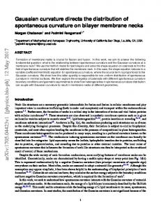
6. Experimental Results The experiments we have done are to use a triangular surface mesh from [8] with 448 faces and 226 vertices as shown in figure 1. The Gaussian curvatures are obtained by the principal curvatures in the original scale. Each time we started an experiment with a random initialization of the configuration. We performed a sequence of tests, and the matching results are summarized in table 1 with curvature disturbance levels up to 5%, 10%, and 50%. Figure 2 shows the Gaussian curvature comparison in different noise levels for the first 20 sites. The matching results show that within 5% of noise level, the node correspondence is 100% correct; for noise level up to 10%, 92% of the correspondence are correct; and for noise level up to 50%, the correct rate is 72%. Running time and iteration numbers are shown in table 2. For curvature noise levels up to 5% and 10%, running time is normally around one minute; for noise level of 50%, it takes several minutes to half an hour to converge. The iteration number for a typical convergence loop is from 25 to 50.

7. Conclusions In this paper, we propose a shape representation framework by using Gaussian curvature and Markov random fields, which can preserve both geometric and topological information of the underlying shape. The experimental results for 3D meshed surface matching are quite promising. Besides matching, the shape representation can also be used for statistical shape analysis, registration, and 3D model in-

Figure 1. Triangular Mesh

Gaussian Curvature

Gaussian Curvature Comparison (noise level: 5, 10, and 50%) 25 original 5% noise 20 10% noise 50% noise 15 10 5 0 −5

0

5

10 Site Number

15

20

Figure 2. Curvature Comparison

dexing and retrieval. Future work will investigate the efficiency of the inference procedure.

Acknowledgements National ICT Australia is funded by the Australian Government’s Backing Australia’s Ability initiative, in part through the Australia Research Council. We wish to thank Cindy Grimm and Timothy D. Gatzke for letting us to use their data sets.

References [1] S. Belongie, J. Malik, and J. Puzicha. Shape matching and object recognition using shape contexts. IEEE Transactions on Pattern Analysis and Machine Intelligence, 24(24):509– 522, 2002.

[2] P. J. Besl and N. D. McKay. A method for registration of 3-d shapes. IEEE Transactions on Pattern Analysis and Machine Intelligence, 14(2):239–256, 1992. [3] P. Bremaud. Markov Chains: Gibbs Fields, Monte Carlo Simulation, and Queues. Springer, 1999. [4] A. M. Bronstein, M. M. Bronstein, A. Spira, and R. Kimmel. Face Recognition from Facial Surface Metric, chapter Computer Vision - ECCV 2004, pages 225–237. Lecture Notes in Computer Science. Springer Berlin / Heidelberg, 2004. [5] Y. Chen and G. Medioni. Object modeling by registration of multiple range images. In Proceedings of the 1991 IEEE International Conference on Robotics and Automation, volume 3, pages 2724–2729, 1991. [6] G. Dudek and J. K. Tsotsos. Shape representation and recognition from multiscale curvature. Computer Vision and Image Understanding, 68(2):170–189, November 1997. [7] F.Cazals and M.Pouget. Estimating differential quantities using polynomial fitting of osculating jets. In Eurographics Symposium on Geometry Processing, volume 3, pages 177– 275, 2003. [8] T. Gatzke and C. Grimm. Tech report wucse-2004-9: Improved curvature estimation on triangular meshes. Technical report, Washington University in St. Louis, September 2003. [9] T. Gatzke, C. Grimm, M. Garland, and S. Zelinka. Curvature maps for local shape comparison. In Proceedings of the IEEE Conference on Shape Modeling and Applications, pages 244–253, June 2005. [10] S. Gold and A. Rangarajan. A graduated assignment algorithm for graph matching. IEEE Transactions on Pattern Analysis and Machine Intelligence, 18(4):377–388, April 1996. [11] L. Gorelick, M. Galun, E. Sharon, R. Basri, and A. Brandi. Shape representation and classification using the poisson equation. In Proceedings of the IEEE Computer Society Conference on Computer Vision and Pattern Recognition (CVPR’04), volume 2, pages II61–II67, 2004. [12] C. Grimm and J. Hughes. Modeling surfaces of arbitrary topology using manifolds. In Proceedings of the 22nd annual conference on Computer graphics and interactive techniques, pages 359–368, 1995. [13] S. Hermann and R. Klette. A comparative study on 2d curvature estimators. Technical report, University of Auckland, June 2006. [14] S. Ho and G. Gerig. Scale Space Methods in Computer Vision, chapter Scale-Space on Image Profiles about an Object Boundary, pages 564–575. Lecture Notes in Computer Science. Springer Berlin / Heidelberg, 2003. [15] D. Hoffman and W. Richards. Parts of recognition. Cognition, to appear, December 1983. MIT Artificial Intelligence Laboratory. [16] D. F. Huber and M. Hebert. A new approach to 3-d terrain mapping. In Proceedings of the 1999 IEEE/RSJ International Conference on Intelligent Robots and Systems, volume 2, pages 1121–1127, 1999. [17] A. E. Johnson and M. Hebert. Using spin images for efficient object recognition in cluttered 3d scences. IEEE Transactions on Pattern Analysis and Machine Intelligence, 21(5):433–449, May 1999.

[18] M. Kazhdan, T. Funkhouser, and S. Rusingkiewicz. Rotation invariant spherical harmonic representation of 3d shape descriptors. In Proceedings of the Eurographics Symposium on Geometry Processing, pages 156–164, 2003. [19] J. J. Koenderink. The structure of images. Biological Cybernetics, 50:363–370, 1984. [20] J. M. Lee. Introduction to Smooth Manifolds. Springer, 2003. [21] S.-M. Lee, A. L. Abbott, N. A. Clark, and P. A. Araman. A shape representation for planar curves by shape signature harmonic embedding. In Proceedings of the IEEE Computer Society Conference on Computer Vision and Pattern Recognition (CVPR’06), volume 2, pages 1940–1947, 2006. [22] P. Liang and J. S. Todhunter. Representation and recognition of surface shapes in range images: A differential geometry approach. Computer Vision, Graphics, and Image Processing, 52(10):78–109, 1990. [23] T. Lindeberg. Scale-Space Theory in Computer Vision. Kluwer Academic Publishers, 1994. [24] C. Lu, S. M. Pizer, and S. Joshi. Scale Space Methods in Computer Vision, chapter A Markov Random Field Approach to Multi-scale Shape Analysis, pages 416–431. Lecture Notes in Computer Science. Springer Berlin / Heidelberg, 2003. [25] B. Luo and E. R. Hancock. Structural graph matching using the em algorithm and singular value decomposition. IEEE Transactions on Pattern Analysis and Machine Intelligence, 23(10):1120–1136, October 2001. [26] S. J. Maybank. Detection of image structures using the fisher information and the rao metric. IEEE Transactions on Pattern Analysis and Machine Intelligence, 26(12):1579–1589, December 2004. [27] S. J. Maybank. The fisher-rao metric for projective transformations of the line. International Journal of Computer Vision, 63(3):191–206, April 2005. [28] G. Medioni and Y. Yasumoto. Corner detection and curve representation using cubic b-splines. In Proceedings of the IEEE Conference on Robotics and Automation, volume 3, pages 764–769, 1986. [29] W. Mio, D. Badlyans, and X. Liu. A computational approach to fisher information geometry with applications to image analysis. In A. Rangarajan, B. C. Vemuri, and A. L. Yuille, editors, EMMCVPR, volume 3757 of Lecture Notes in Computer Science, pages 18–33. Springer, 2005. [30] F. Mohanna and F. Mokhtarian. An efficient active contour model through curvature scale space filtering. Multimedia Tools and Applications, 21:225–242, 2003. [31] F. Mokhtarian, S. Abbasi, and J. Kittler. Indexing an image database by shape content using curvature scale space. In Proceedings of IEE Colloquium on Intelligent Image Databases, pages 4/1–4/6, May 1996. [32] F. Mokhtarian, S. Abbasi, and J. Kittler. Robust and efficient shape indexing through curvature scale space. In BMVC. British Machine Vision Association, 1996. [33] F. Mokhtarian and M. Bober. Curvature Scale Space Representation: Theory, Applications, and MPEG-7 Standardization. Kluwer Academic Publishers, 2003.

[34] A. Peter and A. Rangarajan. Shape analysis using the fisherrao riemannian metric: Unifying shape representation and deformation. IEEE International Symposium on Biomedical Imaging (ISBI), pages 1164–1167, April 2006. [35] I. E. Rube, M. Ahmed, and M. Kamel. Wavelet approximation-based affine invariant shape representation functions. IEEE Transactions on Pattern Analysis and Machine Intelligence, 28(2):323–327, February 2006. [36] D. Saupe and D. V. Vranic. 3d model retrieval with spherical harmonics and moments. In Proceedings of the 23rd DAGM Symposium, pages 392–397, September 2001. [37] S.Geman and D.Geman. Stochastic relaxation, gibbs distributions and the bayesian restoration of images. IEEE Transactions on Pattern Analysis and Machine Intelligence, 6:721–741, 1984. [38] M. Spivak. A Comprehensive Introduction to Differential Geometry, volume 3. Publish or Perish, Inc, 2005. [39] Q. M. Tieng and W. W. Boles. Recognition of 2d object contours using the wavelet transformzero-crossing representation. IEEE Transactions on Pattern Analysis and Machine Intelligence, 19(8):910–916, August 1997. [40] J. van der Poel, C. W. D. de Almeida, and L. V. Batista. A new multiscale, curvature-based shape representation technique for image retrieval based on dsp techniques. In Proceedings of the Fifth International Conference on Hybrid Intelligent Systems, pages 373–378, 2005. [41] S. Wang, Y. Wang, M. Jin, X. Gu, and D. Samaras. 3d surface matching and recognition using conformal geometry. In Proceedings of the IEEE Computer Society Conference on Computer Vision and Pattern Recognition (CVPR’06), volume 2, pages 2453–2460, 2006. [42] G. Winkler. Image Anslysis, Random Fields and Markov Chain Monte Carlo Methods. Springer, 2003. [43] Q. Yang and S. D. Ma. Matching using schwarz integrals. Pattern Recognition, 32(6):1039–1047, June 1999. [44] C. Zahn and R. Roskies. Fourier descriptors for plane closed curves. IEEE Transactions on Computers, 21(3):269–281, March 1972. [45] D. Zhang. Harmonic Shape Images: A 3D Free-form Surface Representation and Its Applications in Surface Matching. PhD thesis, Robotics Institute, Carnegie Mellon University, Pittsburgh, PA, November 1999. [46] D. Zhang and G. Lu. Content-based shape retrieval using different shape descriptor: A comparative study. In Proceedings of the IEEE International Conference on Multimedia and Expo (ICME’01), pages 1139–1142, August 2001.