1-D and 2-D comparison functions yield a high degree of discrimination for local ..... 723â730. [Online]. Available: citeseer.nj.nec.com/article/mori01shape.html.
Curvature Maps For Local Shape Comparison Timothy Gatzke and Cindy Grimm
Michael Garland and Steve Zelinka
Washington University in St. Louis St. Louis, Missouri, USA Telephone: (314) 935–4576
University of Illinois Urbana-Champaign, Illinois, USA Telephone: (800) 555–1212
Abstract— The ability to identify similarities between shapes is important for applications such as medical diagnosis, object registration and alignment, and shape retrieval. In this paper we present a method, the Curvature Map, that uses surface curvature properties in a region around a point to create a unique signature for that point. These signatures can then be compared to determine the similarity of one point to another. To gather curvature information around a point we explore two techniques, rings (which use the local topology of the mesh) and Geodesic Fans (which trace geodesics along the mesh from the point). We explore a variety of comparison functions and provide experimental evidence for which ones provide the best discriminatory power. We show that Curvature Maps are both more robust and provide better discrimination than simply comparing the curvature at individual points.
I. I NTRODUCTION In this paper we address the problem of local surface similarity, i.e., is a region of a surface the same “shape” as another region? This information is useful for a variety of applications. For example, identifying corresponding regions between two similar surfaces is a necessary first step toward alignment and registration of those surfaces. Previous approaches to local surface matching have either focused on man-made objects, where features are easy to find, or required some type of user interaction to select features. Manual selection of corresponding features and subjective determination of the difference between objects are both time consuming processes requiring a high level of expertise. Our approach automates this process, while still providing the user with control over what aspects of the surface match are important. A. Approach Our approach uses curvature, which is an intrinsic property of the surface, as a base metric. Because curvature is a point metric, it does not provide information about the region around the point. To incorporate local shape information, we define a curvature map around a given vertex v. This curvature map accumulates curvature information from a region around v, and can take one of two forms: A one-dimensional (1-D) map, which only considers the distance from v, or a twodimensional (2-D) map that uses both the distance and the orientation information. Note that using just the curvature at v is the 0-D form of the curvature map function. We investigate various methods of building curvature maps from both mean and Gaussian curvature, and the effect of the
size of the region. We then define a similarity function that compares two curvature maps. B. Contribution In this paper we develop the curvature map and comparison functions for local shape similarity. Curvature maps are robust with respect to grid resolution and mesh regularity. Both the 1-D and 2-D comparison functions yield a high degree of discrimination for local shapes, compared to the 0-D methods which have been used previously. Curvature calculation on discrete meshes is often noisy [1] and not always accurate [2]. Because curvature maps combine curvature information over a region, they are less susceptible to these issues. Section II discusses previous work. In Section III we define curvature maps, including how we calculate curvature, define a local region on the surface, and different similarity measures. In Section IV, we evaluate the various similarity measures using both a test shape with known curvature, and several common meshes. Section V summarizes the conclusions of this study and outlines possible areas for future work. II. P REVIOUS W ORK Similarity measures based on distances between sets of points, feature vectors, histograms, signatures, and graph representations can be found in object recognition, threedimensional model matching, computer vision, feature detection, correspondence, registration, and pose estimation. These methods are primarily global rather than local in nature, i.e., they match entire surfaces. A few of these techniques have been applied to local surface matching; we discuss these in more detail. Shum et al. [3] use the Lp distance between local curvature functions mapped to a semi-regular triangulation of the unit sphere as a local measure; unfortunately, this technique is only applicable to closed surfaces which are topologically spherical. A number of segmentation methods also use curvature, particularly the sign of the curvature [4] [5], isosurfaces and extreme curvatures [6], or watersheds of a curvature function [7] [8] [9]. Watershed algorithms show sensitivity to noise and to the user-specified watershed depth threshold. Splitting the surface into regions still gives only coarse information about the differences between local regions, and small changes to the shape can make large changes in the segmentation.
There have been a few attempts to create local signatures. Planitz et al. [10] propose a signature based on a local region around select vertices. However, the use of distances and angles between normals for points in a local support region makes this method sensitive to point distributions. Shape contexts [11] represent the shape of an object, with respect to a particular point on the object, as a 2-D histogram of the relative coordinates of other points sampled from the surface. The sampling of points limits this method for detailed shape matching. These similarity measures are applicable to coarse shape matching for shape retrieval, but generally provide limited discrimination between similar shapes. Moreover, in general, methods based on distances between points, such as Hausdorff distance, multi-resolution Reeb graphs [12], shape distributions [13] [14], and spin images [15], are sensitive to the distribution of the points.
Test surface with rings marked Color coding for the first 9 rings around Vertex A
Vertex B
Vertex A
III. C OMPARING L OCAL S URFACE S HAPE This section describes the Curvature Map, and how it is used to identify regions of similar shape. We first define two methods for creating samples around the point, one based on the mesh topology and one based on geodesic sampling. Next, we describe how we calculate curvature on the mesh. Finally, we define the comparison function itself. A. Defining Rings of a Mesh Given a specified vertex of the mesh, we can define a set of “rings” around the vertex using the existing mesh structure. The ith ring around Vertex v0 is defined as the set of vertices v ∈ V such that there exists a shortest path from v0 to v containing i edges. The set of rings Ri , i ≤ N defines the N -Ring neighborhood about v0 . Figure 1 shows the first nine rings around a selected vertex of the mesh. The ring structure can be extended an arbitrary distance from any point; however, as the distance increases, the shape of the ring may become irregular. B. Geodesic Fans Geodesic fans [16] represent a local surface resampling that provides a uniform neighborhood structure around a vertex. In particular, a geodesic fan consists of a set of spokes, and a set of samples on each spoke. The spokes are geodesics marched out across the surface from the neighborhood center, equally spaced in the conformal plane of the neighborhood’s 1-ring. With the samples equally spaced along each spoke, they form a local geodesic polar map around the vertex. Each set of points equi-distant from the neighborhood center is treated as a ring. Following Zelinka and Garland, we use interpolated normal geodesics [17] where possible, reverting to straightest geodesics [18] if the smoothness criterion for interpolated normal geodesics is not met. We use this procedure to generate fans at each vertex of the mesh. Sample fans at two vertices are shown in Figure 2. Each fan point is defined in terms of the Barycentric coordinates in some triangular face in the original mesh. These Barycentric
Fig. 1. Test surface with Vertices A and B highlighted. The first nine rings defined around Vertex A are color coded. The mesh is fairly uniform except for blending between sections. Note that the ring structure is still well-defined in spite of the skewness near its right edge.
coordinates are used to interpolate curvature values defined on the mesh to the fan point. This forms a uniform sampling of curvature data around each vertex. As the sampling increases, more overhead is required to store the fan data. The regularity of geodesic fans can break down as the distance from the point increases, due to a) stretching of the circumferential spacing while the radial spacing remains uniform, and b) issues in constructing geodesics over longer distances. As a result, the fan resolution may be locally finer, coarser, or both, when compared to the mesh resolution. If the sampling is coarser than the mesh triangle size, then the geodesic fan will not incorporate all of the curvature data available. C. Estimating Curvature Gatzke and Grimm [2] evaluate various curvature estimation methods for triangular meshes. Based on their results, we choose an algorithm that fits a 2-Ring neighborhood using a natural parameterization of the input mesh [19]. This method is reasonably robust with respect to noise as well as mesh irregularity, and provides consistent accuracy of the curvature values. Gaussian curvature and mean curvature are plotted as scalar properties on the surface of the test shape in Figure 3. D. 1-D Curvature Maps The 1-D form of the curvature map is defined over M rings, where the rings come from either the mesh structure or the geodesic fan structure. Each point pi in the map is constructed from data accumulated along the ring Ri . The point pi can have one or more data values; this allows us to compare, for example, both the Gaussian and the mean
Geodesic Fans for vertices A and B (20 spokes, 11 points per spoke)
Vertex B
= {f j : ri →