Neural Networks PERGAMON
Neural Networks 12 (1999) 513–518
Contributed article
An NN-based approach for tuning servocontrollers Elder M. Hemerly*, Cairo L. Nascimento Jr Instituto Tecnolo´gico de Aerona´utica, CTA-ITA-IEEE, 12228-900 Sa˜o Jose´ dos Campos, Sa˜o Paulo, Brazil Received 27 June 1997; received in revised form and accepted 26 October 1998
Abstract Neural networks (NN) are used in this paper to tune PI controllers for unknown plants, which may be nonlinear or open-loop unstable. A simple algorithm, which requires only knowledge of the plant output response direction, is used for training an NN controller, by employing the error between the reference and the plant output. Once this controller achieves good performance, its input–output behavior is approximated by a controller with PI structure, thereby enabling the computation of proportional and integral gains. These gains are familiar to process engineers and can be directly inserted into most existing softwares for process control in industry. Computer simulations on an unstable nonlinear plant and experimental results on a thermal plant are presented to illustrate the usefulness of the proposed approach. 䉷 1999 Elsevier Science Ltd. All rights reserved. Keywords: Adaptive control; PI controller; Backpropagation; Digital control; Neural network; Process control
1. Introduction The vast majority of industrial control loops still rely on the ubiquitous PID controller (Seborg, 1994). The derivative term is not widely used however, hence over 90% of the industrial controllers are of the PI type (Ho et al., 1995). This explains the plethora of techniques for tuning PI controllers. For older ones, see Ziegler and Nichols (1942), Cohen and Coon (1953); and newer ones can be found in Hang et al. (1991) and Hemerly (1991). These techniques are usually derived assuming the controlled plant behaves like a first order plus dead-time model. In Hemerly (1991) any model is allowed for, but the designer has to identify the plant before tuning the controller. Recently, neural networks (NN) appeared as promising tools for designing high performance control systems, for they have the potential for dealing with unfavorable scenarios, owing to nonlinear dynamics, drift in plant parameters and shifts in operating points (see Narendra and Parthasarathy, 1990; Cui and Shin, 1993; Rovithakis and Christodoulou, 1994; Chen and Khalil, 1995 for details). As in the previous four references and similar approaches, in this work we intend to exploit the NN ability to approximate any continuous mapping through learning (Cybenko, 1989). However, in contrast to existing approaches, here we assume the NN-controller is used only for a transient period, * Corresponding author. Fax: 00 55 21 340 5878. E-mail address:
[email protected] (E.M. Hemerly)
during which its behavior is approximated by that of a PI controller. The advantages of this procedure are threefold: 1. the global stability analysis of the control system with NN-controller, which is a complicated problem to deal with, see Chen and Khalil (1995) for instance, can be partly side-stepped for the controller is meant to be used for a finite period of time and under supervision; 2. instead of providing the user with weights connecting nodes in a given NN topology, whose interpretation is far from straightforward, our approach provides proportional and integral gains of a PI controller, which are familiar to process engineers and, as we mentioned before, can be directly inserted into most existing softwares for process control in industry; and 3. the proposed approach can work even when traditional methods fail. For instance, all methods based on step response require the process to be open loop stable. As example of such methods we can mention the classical Ziegler–Nichols method and even the methods used by some industrial controllers, like Foxboro EXACT and Honeywell UDC 6000. For more details, see Astro¨m et al. (1993). The contribution of this paper lies, therefore, in the development of a technique which encapsulates some benefits of NN in a way which is easy to understand and widely used in practice. The reminder of this paper is organized as follows: in Section 2 we summarize the NN-controller presented in
0893-6080/99/$ - see front matter 䉷 1999 Elsevier Science Ltd. All rights reserved. PII: S0893-608 0(98)00147-6
514
E.M. Hemerly, C.L. Nascimento Jr / Neural Networks 12 (1999) 513–518
desired output yd(t). We can then define
Fig. 1. Basic structure of the NN-based control system.
Cui and Shin (1993), which is suitable for our purposes, since the controller is serially connected to the controlled plant. In Section 3 we present the procedure for approximating the NN-controller by a PI controller. In Section 4 we present simulation and experimental results to illustrate the validity of our approach. Conclusions are presented in Section 5.
2. Direct adaptive control via NN
ey
t yd
t ⫺ y
t
system output error;
3
eu
t ud
t ⫺ u
t
control input error
4
where eu(t) is also the network output error. Usual training algorithms rely on (4). In this case, however, such an error is not available for the plant is assumed unknown. If (4) were known, we could use a multilayer perceptron and the backpropagation algorithm for adjusting the NN weights. Assume an NN with N layers, and let F (L), 1 ⬍ L ⬍ N, be the output vector of the Lth hidden layer; F (1) the excitation vector; F (N) the output vector; Q
L i ; 1 ⬍ L ⱕ N, the 1xp (L⫺1) vector of weights at the input of the ith neuron in the Lth layer; B
L i ; 1 ⬍ L ⱕ N, the scalar bias in the ith neuron of the Lth layer. Then by using tanh(.) as squashing function, we have the following algorithm for adjusting weights and biases in the Lth layer, 1 ⬍ L ⬍ N,
L
L⫺1 ^
L Q^
L
t; ij
t ⫹ 1 Q ij
t ⫹ hdi
tFj
5
L ^
L B^
L i
t ⫹ 1 Bi
t ⫹ hdi
t
6
where
Most approaches for adaptive control using NN are indirect, i.e., requires an identification step, in which the NN is trained to attain the same dynamic behavior as the controlled plant. See Chen and Khalil (1995) for instance. The main difficulty in designing direct schemes, namely which adjust the weights based on the error between the reference and the plant output, lies in the fact that the desired NN output is not known beforehand, since the plant is unknown. A direct adaptive scheme using NN is presented in Cui and Shin (1993), where the aforementioned problem is circumvented by supposing the controlled plant is monotone responded, i.e., the derivative of the plant output with respect to its input has always the same sign. This direct scheme is now summarized. The controlled plant is described by _ f
x; u; t; x
t
x 僆 Rn ; u 僆 Rm ;
1
y
t g
x; u; t;
y 僆 Rl
2
and the desired control ud(t) is the one which yields the
L
L 2 d
L i
t ei
t
1 ⫺
Fi
t
7
and e
L i
t
⫹ 1 p
L X
d
L⫹1
tQ^
L⫹1
t l li
8
l1
with boundary condition e
N i
t network output error:
9
The main contribution of Cui and Shin (1993) is to prove that the previous algorithm can be used even if (9) is not known, provided we know the sign of 2yi
t=2uj
t; the (i, j)th component of the Jacobian matrix of the controlled plant. This assumption is not too restrictive in industrial applications, since it is satisfied, for instance, by linear systems cascaded with time delay, dead zone and/or saturation. Additionally, the adaptive control problem is considerably simplified, since explicit identification of the plant is not required. In Section 3 we build on the simplicity of this direct scheme for adaptive control, aiming at tuning a PI controller. 3. Tuning of the pi controller
Fig. 2. NN-based control system with reference model.
In this section we describe how the direct adaptive control scheme, presented in Section 2, can be used for tuning a PI controller. Two structures for direct adaptive control, assuming SISO plants, were investigated. The first one is shown in Fig. 1. The input layer has six nodes, and the previous values of the reference aim at avoiding a too large control signal,
E.M. Hemerly, C.L. Nascimento Jr / Neural Networks 12 (1999) 513–518
515
have " # kp A B ki where " A and B
Fig. 3. Reference and system response with NN controller.
which might cause actuator saturation, when yref
k is discontinuous. Extensive simulations suggested three layers (one input, one hidden, one output) would be enough, with three nodes in the hidden layer. Implementation of this topology in a PC 486-DX2 revealed the computation time for weights and biases update to be smaller than 200 ms. The second structure is shown in Fig. 2, where the reference signal is the output of a reference model, typically second order, with prescribed damping factor j and natural frequency wn. In Fig. 2 we can shape the control effort by selecting a convenient reference model. See Hemerly (1991) for further details. The network in Fig. 2 has three layers, with one node in the hidden layer. Hence we have an extremely simple NN-controller. We now turn our attention to the tuning of the PI controller, by using the structures in Figs. 1 or 2. At time k, we approximate the NN-controller behavior by that of a digital PI controller, described by u
k u
k ⫺ 1 ⫹ kp
e
k ⫺ e
k ⫺ 1 ⫹ ki e
k
10
and since the NN weights and biases can change with time, it is advisable to employ more than just one data point to perform the calculation of kp and ki. Here we consider only the case in which two data points are used. In this case we
Fig. 4. Evolution of kp(t) and ki(t) for Fig. 3.
11
De
k ⫹ De
k ⫺ 2
e
k ⫹ e
k ⫺ 2
De
k ⫺ 1 ⫹ De
k ⫺ 3 e
k ⫺ 1 ⫹ e
k ⫺ 3 "
Du
k ⫹ Du
k ⫺ 2 Du
k ⫺ 1 ⫹ Du
k ⫺ 3
#
12
# :
13
The computation of the proportional and integral gains accordingly to (11) is only possible if A is full rank. This was expected, for in steady state a PI controller is indistinguishable from a P controller. This also ties up with the fact that all approaches for tuning PI controllers, based on pattern recognition, also requires enough excitation. Therefore (11) should be particularly employed when the reference signal undergoes a considerable change. 4. Simulations and real time results In this section we present simulations and real time results employing the approach in Section 3. We consider first simulation results on a nonlinear open-loop unstable plant, and then real time results on a thermal process. A 486-DX2 microcomputer was used in both cases. 4.1. Simulation results Simulations were performed with the nonlinear openloop unstable plant, see Tseng and Hwang (1993) for details, _ x
t ⫺ tan⫺1
u
t; x
t
14
y
t x
t ⫹ exp
⫺1 ⫹ sin
x
t
15
which is used here because all approaches for tuning PI controllers using open loop pattern extraction would fail in this case. It is easy to show that the system (14) and (15) is monotone responded, hence the necessary condition for stability under the direct adaptive scheme in Section 3 is satisfied. By using the structure shown in Fig. 1, and by setting x(0) 0.2, T 0.01 s, h 0.05, we got the result shown in Fig. 3. At the beginning the weights and biases are not appropriate, hence the plant output y(t) deviates considerably from the reference signal yref
t. As time goes on, the NN-controller improves its parameters and reduces the tracking error. By using the procedure described in Section 3 and the data in Fig. 3 for calculating the kp and ki gains, their estimates evolved as shown in Fig. 4. In order to gauge how successful the tuning procedure
516
E.M. Hemerly, C.L. Nascimento Jr / Neural Networks 12 (1999) 513–518
Fig. 5. Performance of PI controller with kp 23.197 and ki 1.748, corresponding to kp (1500) and ki (1500) in Fig. 4.
was, we simply select the last values of kp and ki in Fig. 4 and design a PI controller with these gains. The ensuing performance is shown in Fig. 5. From the aforementioned simulation results, we conclude that the tuning procedure performed well. The PI controller in Fig. 5 has acceptable performance, and it is quite similar to that obtained with the NN controller in Fig. 3, once the NN parameters has converged to appropriate values. 4.2. Real time results We consider the Feedback’s process trainer PT326, see Fig. 6, which is a thermal process in which air is fanned through a polystyrene tube and heated at the inlet, by a mesh of resistor wires. The air temperature is measured by a thermocouple at the outlet. We consider first the case in which the NN controller in Fig. 1 is used. By selecting T 0.2 s and h 0.005, we got Fig. 7, which corresponds to a typical realization, since the plant output is quite noisy. The plant output, in Fig. 7, is sluggish at the beginning, but improves progressively. The estimates of the proportional and integral gains are shown in Fig. 8. By designing a PI controller with the last values of the
Fig. 6. Set-up for real time application.
Fig. 7. Reference and system response with NN controller as in Fig. 1.
proportional and integral gains in Fig. 8, we got the performance shown in Fig. 9. The performance in Fig. 9 is acceptable. It is worth mentioning that the plant response is not symmetric because the cooling and heating dynamics are different. It should be stressed that in Fig. 1 the NN controller is trying to minimize the tracking error. This can result in too large control signals, mainly when the reference is step like. In order to smoothen the control signal, we now use the NN controller shown in Fig. 2. By selecting j 0.65 and wn 0.8 rad/s, Fig. 10 was obtained. The estimates of the proportional and integral gains are shown in Fig. 11, and the performance obtained with the PI controller is displayed in Fig. 12. We conclude the PI controller is able to almost zero the tracking error between the reference and plant output.
5. Conclusion A simple approach for tuning PI controllers using direct adaptive control via NN was proposed in this paper. Only the plant output response direction is required, besides the fact that the plant can be stabilized with a PI controller, and the approach can be used with nonlinear or open-loop unstable plants, which are not easily handled, if at all, by other tuning approaches. Therefore, the proposed approach enhances the applicability of NN in control problems, since
Fig. 8. Evolution of kp(t) and ki(t) for Fig. 7.
E.M. Hemerly, C.L. Nascimento Jr / Neural Networks 12 (1999) 513–518
Fig. 9. Performance of PI controller with kp 1.128 and ki 0.161, corresponding to kp (500) and ki (500) in Fig. 8.
the tuning of PI controllers is a basic problem in industrial applications. It would be highly desirable to automate the tuning process, but this would depend on ensuring global stability of the closed loop system, which is a topic undergoing intensive research and there is no general result available in the literature yet, see Appendix. Hence the approach presented here should be used on request, as is the case with other approaches. However, only the first time the PI controller is tuned requires particular care. From then on, in case the plant dynamics changes, we already have favorable initial values for the NN parameters, hence the tuning procedure will be much faster and reliable. Acknowledgements This work was sponsored by CNPq-Conselho Nacional de Desenvolvimento Cientı´fico e Tecnolo´gico, under grants 300158/95-5(RN) and 522389/94-5. Appendix. Stability for NN controller The global stability of the control systems presented in Figs. 1 and 2, with three-layer NN type, has not been proved yet, as far as we are aware. The strongest stability result available seems to be the one provided by Yabuta and
517
Fig. 11. Evolution of kp(t) and ki(t) for Fig. 10.
Fig. 12. Performance of PI controller with kp 2.411 and ki 0.276, corresponding to kp (500) and ki (500) in Fig. 11.
Yamada (1992). Via a local analysis it is shown that the stability using the backpropagation method depends on both the initial value of the weight vector and the gain tuning parameter h in (5). For a two-layer NN type, which is linear in the tuning parameters, stronger results are available. For instance, in Jagannathan and Lewis (1996) it is shown that global stability is ensured by using the delta-rule-based update term plus a correction similar to the e-modification (used in conventional adaptive control of continuous linear systems). It is worth stressing that this modified tuning rule, although more complicated and less appealing than the backpropagation method, could also were used here, for the procedure for mapping the NN controller to a PI one relies only on the NN input/output values.
References
Fig. 10. Reference and system response with NN controller as in Fig. 2, with j 0.65 and wn 0.8 rad/s.
Astro¨m, K. J., Ha¨gglund, T., Hang, C. C., & Ho, W. K. (1993). Automatic tuning and adaptation for PID controllers – a survey. Control Eng. Practice, 1 (4), 699–714. Chen, F. -C., & Khalil, H. K. (1995). Adaptive control of a class of nonlinear discrete-time systems using neural networks. IEEE Trans. Auto. Control, 40 (5), 791–801. Cohen, G. H., & Coon, G. A. (1953). Theoretical consideration of retarded control. Trans. ASME, 75, 827–834. Cui, X., & Shin, K. G. (1993). Direct control and coordination using neural networks. IEEE Trans. Syst., Man, and Cybern., 23 (3), 686–697.
518
E.M. Hemerly, C.L. Nascimento Jr / Neural Networks 12 (1999) 513–518
Cybenko, G. (1989). Approximation by superpositions of a sigmoid function. Math. Control, Signals, and Systems, 2 (4), 303–314. Hang, C. C, Astro¨m, K. J., & Ho, W. K. (1991). Refinements of the Ziegler–Nichols tuning formula. IEE Proc. Part D, 138 (2), 111–118. Hemerly, E. M. (1991). PC-based packages for identification, optimization and adaptive control. IEEE Control Systems Magazine, 11 (2), 37–43. Ho, W. K., Hang, C. C., & Zhou, J. H. (1995). Performance and gain and phase margins of well-known pi tuning formulas. IEEE Trans. Control Syst. Technology, 3 (2), 245–248. Jagannathan, S., & Lewis, F. L. (1996). Discrete-time neural net controller for a class of nonlinear dynamical systems. IEEE Trans. Automatic Control, 41 (11), 1693–1699. Narendra, K. S., & Parthasarathy, K. (1990). Identification and control of
dynamical systems using neural networks. IEEE Trans. Neural Networks, 1 (1), 4–27. Rovithakis, G. A., & Christodoulou, M. A. (1994). Adaptive control of unknown plants using dynamical neural networks. IEEE Trans. Syst., Man, and Cybern., 24 (3), 400–412. Seborg, D. E. (1994). A perspective on advanced strategies for process control. Modelling, Identification and Control, 15 (3), 179–189. Tseng, H. C., & Hwang, V. H. (1993). Servocontroller tuning with fuzzy logic. IEEE Trans. Control Syst. Technology, 1 (4), 262–269. Yabuta, T., & Yamada, T. (1992). Neural network controller characteristics with regard to adaptive control. IEEE Trans. Syst., Man, and Cybern., 22 (1), 170–176. Ziegler, J. G., & Nichols, N. B. (1942). Optimum settings for automatic controllers. Trans. ASME, 64, 759–768.