per, we describe an extension of the graphical program- ming tool that allows the user to interactively optimize a 1D functional of the output of the data-flow ...
Proc. IEEE Int. Conf. on Image Processing, Vol. III, pp. 826-830, Austin, TX, November 13-16, 1994.
AN OBJECT-ORIENTED OPTIMIZATION SYSTEM G. S. Cunningham, K. M. Hanson, G. R. Jennings, Jr., and D. R. Wolf Los Alamos National Laboratory, MS P940 Los Alamos, New Mexico 87545 USA {cunning, kmh} @lanl.gov ABSTRACT We describe the implementation of a graphical programming tool in the object-oriented language, Smalltalk80, that allows a user to construct a radiographic measurement model. The measurement model can be used to generate the measurements predicted by a given parameterized model of an experimental object. We also describe extensions to the graphical programming tool that allow it to be used to perform Bayesian inference on very large sets of object parameters, given actual experimental data, by optimizing the likelihood or posterior probability of the parameters, given the actual data. 1. INTRODUCTION The object-oriented (OO) paradigm has recently attracted attention because of its promise for code reuse and ease of maintainence, in addition to the natural and intuitive language it promotes for discussion of software [?]. We have built and described an OO graphical programming tool [?] that allows a user to connect icons, which represent data transforms, on a canvas in order to define a data-flow diagram that acts on a user-defined object parameterization. In this paper, we describe an extension of the graphical programming tool that allows the user to interactively optimize a 1D functional of the output of the data-flow diagram with respect to object parameters. We discuss the advantages of programming the optimization tool in an OO language. We believe that the optimization tool will be useful to scientists and engineers for orchestrating Bayesian inference and hypothesis testing of geometric object parameters given actual radiographic data [?]. The general problem for which these tools are intended is the determination of an object of unknown shape and distribution, described by a user-defined parameterization, given limited data generated by a well-characterized, Supported by the United States Department of Energy under contract number W-7405-ENG-36.
826
user-defined measurement system. The graphical programming tool, in conjunction with a likelihood function, allows the user to define a complete model of a measurement system. The maximum likelihood (ML) estimate of the parameters that describe the experimental object can be obtained using the optimization tool. Maximum a posteriori (MAP) estimates can also be obtained, if prior information is used.
2. THE OO PARADIGM The OO paradigm is founded on the concept of an object. Objects have responsibilities, or methods, and data, or attributes. To talk about objects, either to one another in software analysis or design, or to the computer in a programming session, is natural and intuitive, since we think in terms of objects. Attributes are encapsulated by methods so that internal data storage, accessing, and manipulation, is not important to the “outside world”, which can only obtain information about the attributes by messaging the object to perform some method. Encapsulation and messaging facilitate the construction of flexible, easy-to-understand software modules. Classes are templates of objects, and are contained in class hierarchies, wherein subclasses inherit methods and attributes from superclasses, so that code is re-used and sensibly organized. Finally, type-casting is eliminated with the use of dynamic binding. We are using Smalltalk-80 and the VisualWorks programming environment from ParcPlace Systems in conjunction with C, Fortran, and X-Windows. Smalltalk80 is a pure object-oriented programming language, which truly encourages object-oriented thinking. However, its poor performance in executing loops and numerical computations has forced us to use C and Fortran for numerically intensive computations and X-Windows for loop-intensive graphics.
input single-output (Parameter and its subclasses). Parameter and its subclasses define the object model that is the input to the measurement model defined by the data-flow diagram. For example, a GeometricObjectModel has a listOfComponents that might contain a Polygon2D, a Bezier2D, a Grid2D, and a UniformGrid2D. 4. AN OO OPTIMIZER Let the output of the measurement system model specˆ ified by the data-flow diagram be predicted data, d(θ), where θ is a set of parameters that defines the object model. For example, θ = {θij } might be the set of density values in a UniformGrid2D of fixed size. If the user has data, d, that are generated by a measurement system that corresponds well to the measurement system model, plus some additive noise, n, with probability ˆ is a 1D funcdistribution PN (n), then PN (d − d(θ)) tional on the output of the data-flow diagram, called ˆ over the likelihood function. Optimizing PN (d − d(θ)) θ produces the ML estimate of θ given the data, d. If PΘ (θ) is a prior probability distribution over θ, then ˆ φ(θ) = log[PN (d − d(θ))] + log[PΘ (θ)] is a 1D functional called the log posterior. Maximizing φ(θ) over θ produces the MAP estimate of θ, given the data, d. Thus, the capability for optimizing 1D functionals of data-flow diagrams includes the capability for solving Bayesian inference problems. We have extended the graphical programming tool to include Gaussian likelihood functions and the ability to optimize them with respect to object-model parameters using conjugate gradient (for unconstrained problems) and gradient descent (for constrained problems) methods.
Figure 1: The canvas for the graphical programming tool. 3. AN OO GRAPHICAL PROGRAMMING TOOL Figure 1 shows a typical example of the graphical programming tool, which operates as follows. The user is presented with a canvas, on which appear buttons that allow the user to add items to, or delete items from, the canvas. The user can add or delete Transforms and Connections. Transforms map input Data to output Data and are represented on the screen by an icon. The user specifies the data-flow by connecting one Transform to another using a Connection, which is represented on the screen as a set of connected line segments. The Transforms are “living” objects and the user can interact with them in several ways. He can see a description of a Transform and change the parameters that define it. The user can also message the Transform to display its output. This message is forwarded to the Transform’s output attribute, which is messaged to display itself. The fact that the Transform objects are alive distinguishes this graphical programming tool from one that allows a user to construct and visualize a script that contains a sequence of actions to be executed in a certain order. We have written classes for several categories of Transforms, including MultiInputSingleOutput (Add, Multiply, Subtract), SingleInputSingleOutput (Convolution, Exponential, Log, Log10, SqRt, Sin, Cos, LineIntegral, ParallelLineIntegral) and no-
4.1. The reverse adjoint method We obtain the gradient of the log likelihood with re∂φ ) using a reverse spect to object model parameters ( ∂θ i adjoint technique, which implements the chain-rule for differentiation from back to front [?]. For example, let us define a simple measurement ˆ model, such as that shown in Fig. 1, wherein d(x) denotes the data predicted by taking line integrals of a UniformGrid2D object model, x, using transform L, to produce pathlengths, y, which are then pointwise exponentiated to produce attenuations, z, and convolved with a point spread function represented by the matrix ˆ H to finally produce d(x). Then ˆ = H(E(L(x))) d(x) 827
(1)
is an approximation to a true radiographic measurement system that can be easily built using the graphical programming tool. If our actual data are d, and we assume that they are produced by adding white gaussian noise to the data predicted by the true object xTRUE , then φ is just the norm of dˆ − d, and the derivative of φ w.r.t. dˆ is just d∗ = 2(dˆ − d). The derivative of φ w.r.t. z is just z ∗ = H T d∗ , that is, the adjoint operator for the Convolution acting on the the Data passed back to it by the Likelihood. Similarly, the derivative of φ w.r.t. y is just y ∗ = − exp−y ·z ∗ = EyT z ∗ , where · is pointwise multiplication and y is the current input to the Exponential. Finally, the derivative of φ w.r.t. the object parameters x can be obtained by “backprojecting” the adjoint Data y ∗ to produce x∗ = LT y ∗ . Thus, the derivative of φ w.r.t. x can be written: �φ = LT (EyT (H T (2(dˆ − d))))
eventually returns the gradient of the Likelihood with respect to itself. Connections are also modified in order to propogate Data in both directions. When a Connection is told to getData it gets the Data from the previous Transform and sends it to the one upstream requesting it for input. When a Connection is told to getAdjointData, it gets the adjointData from the Transform upstream and sends it to the Transform downstream, requesting it as an adjointInput. Note that, in general, computing the adjoint gradient operator requires that the Transform know the current state of its input, since the derivative may well depend on the input (the Exponential, e.g.). Thus, it is natural to bundle the Transform with its current state (stored in its input) as we have done. Parameters are given extended responsibilities in order to accomodate the existing optimization strategies. In particular, all Parameters must be responsible for add’ing themselves to and subtract’ing themselves from any instance of the same Class. Parameters also must be able to multiplyByScalar:aScalar, find their norm and determine their innerProductWith:anObject for anObject that is an instance of the same class. Furthermore, we have made some Parameters capable of projecting themselves onto certain constraint sets, namely upper and lower bounds. Since addition, subtraction, multiplication by scalar, norm, inner product, and constraint satisfaction are all the responsibility of Parameters, the Optimizer logic can be applied to very different types of optimizations problems, e.g. one or two-dimensional de-convolution, tomographic inversion, inversion from noisy nonlinear point functions, etc. The logic in the Optimizer can work for any vector space, regardless of its detailed structure. The detailed structure of the Parameters being optimized is taken care of in the implementation of the fundamental vector space operations (addition, multiplication by scalar, etc.). The encapsulation and polymorphism provided by the Parameters allows us to concentrate on building and adapting robust, abstract, optimization algorithms that can be widely employed.
(2)
This equation suggests a “reverse-adjoint” implementation. Each Transform must know how to calculate the derivative of its outputs w.r.t. its inputs. These are the “sensitivity matrices” LT , EyT , H T , which may well depend on the current input state of the Transform. Rather than calculating the sensitivity matrices explicitly and then having them operate on the adjoint Data set passed from the upstream Transform, we write adjoint operator codes that automatically process the adjoint Data set to produce a new adjoint Data set without calculating the sensitivity matrices explicitly. So, for example, we don’t explicitly calculate EyT , which is diagonal but rather use the adjoint Data z ∗ to produce the adjoint Data y ∗ = − exp−y ·z ∗ = E T (y)z ∗ , which only requires a vector multiply. 4.2. Extending the class hierarchy Extending the responsibility of Transforms to include an associated adjoint gradient operation is easily accomodated in our OO programming environment. The adjoint method takes Data that has the structure of a Transform output and maps it into Data that has the structure of a Transform input. Dual to the data-flow mode of operation, where outputs of the data-flow diagram query previous Transforms to generateOutput until eventually Parameters are encountered and just return themselves, in the gradient-flow mode of operation Parameters query forward Transforms to generateAdjointOutput until eventually a Likelihood is encountered and returns the gradient of itself with respect to the present state of its input. Thus, the gradients flow backwards, or in reverse, until each Parameter
4.3. Capabilities The user specifies that a Parameter is to be optimized by connecting it to the Optimizer, as in Fig. 1. The user can specify an optimization strategy (conjugate gradient or gradient descent), tolerances, and maximum number of iterations for the global search and each line minimization, and gets feedback on the current step size, number of global iterations, and the number of likelihood evalutions thus far (see Fig. 2). 828
Figure 2: The interface for the optimizer.
At any point during the optimization, the user can interrupt the Optimizer so that he can see the present state of the solution (and Data predicted by the present solution) by using the graphical programming tool, which contains icons that represent the “live” Data being optimized. The present solution can be modified interactively using modelling tools that are called by interacting with the icon that represents the Parameter of interest. Transforms can also be changed at any time. The log likelihood and likelihood can be plotted as a function of step along the current gradient direction, and the effect of stepping along the gradient from the present solution for various step sizes can be visualized easily. These capabilities are very useful for understanding how the optimization is working, as well as for guiding the Optimizer toward a solution. Note that a “global” derivative of φ w.r.t. object parameters is obtained by “local” message-passing and methods operating on encapsulated data. For example, one can change the fundamental representation of the object described above by having a Polygon2D parameterization θ that feeds into a ConvertToUniformGrid2D Transform to produce a UniformGrid2D x. One can use the previous graphical program as it is, and just insert the new Transform “before” x. Then x∗ , the derivative of φ w.r.t. x, can be backpropogated to produce θ∗ , the derivative of φ w.r.t. θ. The ability to cascade models of the experimental object suggests a “level of detail” approach to optimization (called multiscale if the successfully-refined parameterizations are UniformGrid2Ds with smaller pixels and called multigrid if the parameterizations are successfully-refined ge-
Figure 3: Original object (top) and two reconstructions (bottom) from six noiseless views; without constraints on the left and with minimum- and maximum-value constraints on the right. ometrical descriptions). Finally, the Optimizer can be used to probe the confidence that the user should have in the final solution. The user can select two states of the Parameter set, say P1 and P2 , and ask the Optimizer to provide a one-dimensional plot of the likelihood as a function of the new Parameter set, αP1 + (1 − α)P2 . For example, one could perturb a Polygon2D solution, P1 , by moving a boundary vertex to a new location to produce P2 . Plotting the likelihood as a function of αP1 + (1 − α)P2 would then reveal the confidence one should have in the position of that boundary vertex – a broad likelihood means that there are many positions of the boundary point that are equally likely, and so the position of that vertex should not be trusted. 4.4. An example Two example reconstructions are shown in Fig. 3. The original 128x128 object (on the top) has an attenuation of 6.0 on the interior of its boundary and 0.0 outside. The data used in the reconstruction are obtained by exponentiating the projections from 6 views (256 projection bins per view) and convolving the projections with a gaussian blur function (σ = 4 pixels). No noise is added for this simple demonstration. Both recon-
829
structions use the measurement model in Fig. 1, with the known σ for the blur function. The reconstruction on the bottom left of Fig. 3 is obtained by imposing a non-negativity constraint on the reconstructed attenuation values, and the reconstruction on the bottom right is obtained using non-negativity and an upper bound constraint of 6.0. 5. SUMMARY The advantages of an OO language are enormous in the context of graphical programming, graphical object modeling, and optimization. Not only did the OO paradigm make extending the graphical programming tool to include optimization easier than we expected, it also stimulated our creativity. The potential extensions we envision to interactive, graphical optimization using the foundation we have discussed in this paper are very exciting. Our immediate future plans include extending the 2D radiographic measurement model to 3D polyhedra and volumetric grids. We also plan to incorporate other measurement models, such as range data (that measures exterior surface location) and surface velocity data. Ultimately, we envision 3D time-evolving object and measurement models that will be used to fuse data from a variety of experimental diagnostics. 6. REFERENCES [1] Cunningham, G.S., Hanson, K.M., Jennings, Jr. G.R., Wolf, D.R., “An object-oriented implementation of a graphical programming system,” to be published in Proc. SPIE 2163, 1994. [2] Hanson, K.M., “Bayesian reconstruction based on flexible prior models,” J. Opt. Soc. Am. A 10, 1993, pp. 997-1004. [3] Taylor, D. A., Object-Oriented Technology: A Manager’s Guide, Addison-Wesley, 1990. [4] Thacker, W.C., “Automatic differentiation from an oceanographer’s perspective,” Automatic Differentiation of Algorithms: Theory, Implementation, and Application, ed. A. Griewank and G. Corliss, SIAM, 1991, 360 ff.
830