NOVEMBER 2000
DAVIS ET AL.
1455
An Objective Method for Deriving Atmospheric Structure from Airborne Lidar Observations K. J. DAVIS* Department of Soil, Water, and Climate, University of Minnesota, St. Paul, Minnesota
N. GAMAGE University Corporation for Atmospheric Research, Boulder, Colorado
C. R. HAGELBERG Los Alamos National Laboratory, Los Alamos, New Mexico
C. KIEMLE Lidar Group, Deutsches Zentrum fu¨r Luft- und Raumfahrt, Oberpfaffenhofen, Germany
D. H. LENSCHOW
AND
P. P. SULLIVAN
National Center for Atmospheric Research,1 Boulder, Colorado (Manuscript received 17 June 1999, in final form 18 December 1999) ABSTRACT Wavelet analysis is applied to airborne infrared lidar data to obtain an objective determination of boundaries in aerosol backscatter that are associated with boundary layer structure. This technique allows high-resolution spatial variability of planetary boundary layer height and other structures to be derived in complex, multilayered atmospheres. The technique is illustrated using data from four different lidar systems deployed on four different field campaigns. One case illustrates high-frequency retrieval of the top of a strongly convective boundary layer. A second case illustrates the retrieval of multiple layers in a complex, stably stratified region of the lower troposphere. The method is easily modified to allow for varying aerosol distributions and data quality. Two more difficult cases, data that contain a great deal of instrumental noise and a cloud-topped convective layer, are described briefly. The method is also adaptable to model analysis, as is shown via application to large eddy simulation data.
1. Introduction Both the horizontal and vertical structures of the atmospheric boundary layer (ABL) have traditionally been observed in situ from platforms such as balloons, towers, and aircraft. These observations are generally time series at one or several discrete altitudes. Recently,
* Current affiliation: Department of Meteorology, The Pennsylvania State University, University Park, Pennsylvania. 1 The National Center for Atmospheric Research is sponsored by the National Science Foundation. Corresponding author address: Dr. Kenneth Davis, Department of Meteorology, The Pennsylvania State University, 512 Walker Building, University Park, PA 16802. E-mail:
[email protected]
q 2000 American Meteorological Society
remote sensing technology such as lidar, radar, and sodar have created a flood of nearly continuous range-resolved observations of the atmosphere. Airborne remote sensing instruments, for example, provide nearly instantaneous (compared to typical wind velocities) observations of large, two-dimensional slices of the atmosphere. Three-dimensional numerical models of the atmosphere, in particular large eddy simulations (LESs), provide a wealth of information about the three-dimensional structure of the ABL. These data present new opportunities for understanding ABL structures but also new challenges in data analysis. Our observational focus in this paper is airborne lidar. Lidar (light detection and ranging) is particularly sensitive to changes in atmospheric aerosol concentrations. The basic principles of lidar are described by Measures (1984). The ABL typically contains greater aerosol con-
1456
JOURNAL OF ATMOSPHERIC AND OCEANIC TECHNOLOGY
centrations than the overlying troposphere and hence has larger lidar backscatter. These changes in light backscattering caused by varying aerosol concentration provide a useful tool for remotely observing the two-dimensional structure of the ABL. Typical airborne lidar systems obtain roughly 10-m vertical resolution for each lidar shot and have pulse repetition rates of 5–10 s21 . Typical aircraft velocities of about 100 m s21 result in horizontal data resolution of 10–20 m. Lidars with higher pulse repetition frequencies are likely to become more common in the future. With these high data volumes, objectively extracting atmospheric structure requires robust, automated algorithms. Several authors have used lidar backscatter to derive convective boundary layer (CBL) height. A mean ABL height can be determined by averaging many backscatter profiles and identifying the sharp change that often occurs at the CBL top by eye, as would be done with a radiosonde temperature profile. Piironen and Eloranta (1995) looked at the variance from an ensemble of backscatter profiles and identified the point of maximum variance as the CBL top. This maximum in variance is caused by the convoluted shape of the CBL top and by eddies of entrained air with differing aerosol concentrations. These methods are limited to mean CBL structure. A common method for deriving higher spatially resolved data is application of a simple threshold. Threshold techniques are often used for cloud-base detection using laser ceilometers. This is well suited to cases where the contrast in backscatter is very large but does not provide good precision when the contrast between atmospheric layers approaches the level of instrumental noise, which is often the case for clear-air boundaries such as the top of the ABL or layers associated with a stably stratified atmosphere. In this case incoherent instrument noise can blur subtle but spatially coherent transitions. Complications also arise if the mean level of backscattered power varies from one profile to the next due to instrument performance or changes in atmospheric properties. Melfi et al. (1985) used a simple threshold, and Kiemle et al. (1995) used a maximum gradient in high-resolution backscatter profiles to derive spatial variability in CBL height. When using a gradient approach some vertical and/or horizontal smoothing is usually required prior to differentiation to reduce spurious results due to noise in the backscatter signal. Both the amount of smoothing and the vertical interval over which the signal is differentiated are typically chosen empirically. This method is fairly sensitive to instrumental noise in the backscatter profile. An objective derivation of CBL structure that preserves maximum spatial resolution for less than ideal conditions requires a more robust edgedetection algorithm. Wavelet analysis (Daubechies 1992; Chui 1992; Meyer 1993) has been used for signal and image processing for some time (Mallat 1989; Mallat and Zhong 1992;
VOLUME 17
Mallat and Hwang 1992). The simplest wavelet, the Haar, dates back to 1910 (Daubechies 1992). In meteorology, wavelet analysis has been applied to time series analysis of data from turbulent to climatological timescales (Gamage and Hagelberg 1993; Howell and Mahrt 1994; Foufoula-Georgiou and Kumar 1994). In this paper, we use a Haar wavelet to detect backscatter boundaries in a two-dimensional vertical cross section of lidar observations that includes the ABL. We show that wavelet analysis provides a robust, automated means of deriving high-resolution atmospheric structure using a variety of instruments and under a wide range of atmospheric conditions. The method presented here has been adopted by other investigators and applied in several studies (Kiemle et al. 1997; Davis et al. 1997; Ehret et al. 1996; Russell et al. 1998; Sullivan et al. 1998; Mann et al. 1995; Wang and Lenschow 1995), and a modified version is demonstrated by Cohn et al. (1998) and Cohn and Angevine (2000). This paper documents the technique that has been used in these studies. The technique has several attractive features. It is multiscale; that is, it can retrieve structure at a variety of vertical spatial scales. A focus on larger spatial scales minimizes the influence of incoherent instrument noise on boundary retrieval and identifies the locations of subtle but coherent transitions. The sharpness of the Haar function, however, does not blur the locations of atmospheric transitions as can be the case with smoothing techniques. It can retrieve multiple boundaries from a single lidar profile and segregate the boundaries according to their strength and sign. It treats each profile independently and so is not influenced by shot-to-shot power fluctuations. Finally, the scale capturing the dominant atmospheric structure can be chosen objectively, making the method entirely automated except for the choice of the wavelet. We also show an application of the method to LES potential temperature fields. Analysis of high spatial and temporal resolution model output presents problems similar to the analysis of high-resolution, large volume observational datasets. The application is relatively simple given the absence of instrumental noise and was demonstrated by Sullivan et al. (1998). 2. Method In each of the airborne lidar datasets analyzed, highly detailed atmospheric structure is revealed by a contrast in backscatter. This contrast is due primarily to spatial variability in the aerosol content of the atmosphere. These coherent patterns in lidar backscatter are contaminated (to varying degrees) by uncorrelated instrumental noise. The cases chosen exhibit a variety of spatial scales, backscatter profile shapes, and multiple layers. Examples are shown in Figs. 1 and 2. They are described in more detail in the next section of the text. This section describes the method applied to these data. We objectively retrieve the structural details revealed
NOVEMBER 2000
1457
DAVIS ET AL.
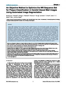
FIG. 1. Lidar backscatter as observed over northern Manitoba using the DLR H 2O differential absorption lidar. Lidar was pointed downward and on board the NCAR Electra research aircraft as part of the BOREAS experiment. High backscatter at the bottom of the image is the ground reflection. Data are range-square corrected relative backscatter. The image shows a very well defined cloud-free convective boundary layer. Universal time is plotted. Local standard time is UTC 2 6 h.
via lidar and identify the scales of atmospheric structure. The method we use is based on the similarity between the sharp, coherent changes in backscatter shown in Figs. 1 and 2, and a step function, also known as the Haar function. The algorithm is applied to a single vertical lidar backscatter profile, then repeated for every profile in the dataset under consideration. Figure 3a contains a single lidar backscatter profile showing coherent, large-scale atmospheric structure overlaid on a background of uncorrelated instrument noise and smaller-scale atmospheric structure. To objectively extract the locations of the atmospheric boundaries in the lidar backscatter profile shown in Fig. 3a, and the thousands of profiles shown in Fig. 1, we study the convolution of a step function, h a,b (z) with the backscatter profile. The step, or Haar function is defined as
1 2
21:
z2b h 5 1: a
a #z#b 2 a b#z#b1 2 b2
(1)
elsewhere, 0: where z represents distance in the vertical in this application, and a and b describe the dilation and translation of the function, respectively.
The convolution or localized transform, Wf (a, b), of the Haar function with the backscatter profile we choose is the covariance transform defined by Gamage and Hagelberg (1993): W f (a, b) 5 a21
E
zt
zb
f (z)h
1
2
z2b dz, a
(2)
where z b and z t are the bottom and top altitudes in the lidar backscatter profile, and f (z) is the lidar backscatter as a function of altitude, z. An example of Wf (a, b) is shown in Fig. 3b. Gamage and Hagelberg (1993) discuss the benefit of the a21 normalization for event-finding algorithms, as opposed to the more common, norm-preserving wavelet transform where a21/2 is the normalization factor. Figure 3b shows the behavior of the covariance transform as a function of both dilation a and translation b. Note the strong maximum at about 1800 m that persists at all wavelet dilations. This corresponds to the strong steplike decrease in backscatter at the top of the convective boundary layer shown in Fig. 3a. Aerosols are trapped in the CBL by a potential temperature inversion at this level. An in situ aircraft sounding for this case is presented by Kiemle et al. (1997). Some smaller-scale structure is evident at moderate dilations (75 and 187 m). The covariance transform at
1458
JOURNAL OF ATMOSPHERIC AND OCEANIC TECHNOLOGY
VOLUME 17
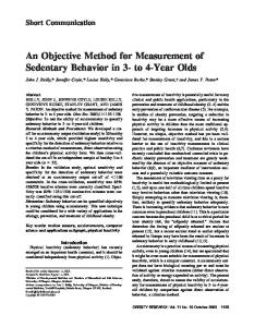
FIG. 2. Lidar backscatter image of the downwind end of the smoke plume emanating from the Kuwait oil fires in 1991 following the Persian Gulf War. Data are range-square corrected and displayed on a logarithmic decibel scale. The Stanford Research Institute lidar was pointed downward from the NCAR Electra research aircraft as part of the KOFSE. The plume originated about 180 km upwind of this image. The mean wind is blowing left to right. The image shows a complex, multilayered structure typical of a stably stratified atmosphere. Time plotted is local standard time.
7.5-m dilation (a two-point difference) is dominated by uncorrelated noise in the lidar backscatter profile. Even the CBL top is difficult to distinguish at this dilation. The covariance transform at minimum dilation (a twopoint difference) is equivalent to the often used gradient technique with no vertical smoothing. Various atmospheric structures could be derived from these covariance transforms by examining the locations of the local maxima and minima. In order to develop an objective methodology, we propose focusing first on the dilation a that has the most dominant boundaries with the characteristic shape of the Haar function h. We choose this dilation by examining the variance of the covariance transform. Figure 3c shows the integral of the covariance transform, Wf (a, b), over all translations, b, for each value of the dilation, a. This quantity, defined by Gamage and Hagelberg (1993) as D 2 (a) 5
E
zt
[W f (a, b)] 2 db,
(3)
zb
is similar to a power spectrum in that it is a measure of the portion of the variance of f (z) at each dilation, a, but with no information about the location of the variance since we have integrated over b. If we had used a norm-preserving wavelet decomposition, the integral
of D 2 (a) over all dilations, a, would equal the variance of f (z). Following Gamage and Hagelberg (1993) we refer to D 2 (a) as the wavelet variance. The maximum in the wavelet variance occurs at the maximum possible dilation, or 1006 m. This dilation of maximum wavelet variance reflects the fact that the CBL is the dominant atmospheric structure in this lidar backscatter profile, and the distance from z t (the maximum altitude of the lidar data) to the CBL top is about equivalent to the maximum possible dilation. We now define an idealized algorithm for objectively determining atmospheric structures as revealed via lidar backscatter. This process is summarized in Fig. 4. Taking a profile like Fig. 3a we calculate the covariance transform Wf (a, b) and the quantity D 2 (a), which is a measure of the variance captured by each dilation, a. We search for the global maximum in D 2 (a). The scale of the maximum in D 2 (a), amax , is the scale of the dominant structures in the lidar backscatter profile. We then search Wf (amax , b) for local maxima and minima. The locations of these maxima and minima, bmax and bmin i i , and the associated values of the covariance transform, Wf (amax , bmax ) and Wf (amax , bmin i i ), are the locations and relative strengths of steplike boundaries in the lidar backscatter profile, f (z). The index i refers to multiple
NOVEMBER 2000
DAVIS ET AL.
1459
FIG. 3. The lower left panel (a) shows one range-square corrected lidar backscatter profile (arbitrary units) from the DLR lidar during the BOREAS experiment. This figure captures a single lidar shot from data shown in Fig. 1. Dashed horizontal lines indicate the location of the global maximum in the covariance transform [see Eq. (2)] at the dilation of maximum variance. The upper panel (b) shows the covariance transform for a range of wavelet dilations and translations applied to the backscatter profile. The horizontal dashed line is the same as in the backscatter plot, and the dilation of maximum covariance (a 5 1006 m) is shown in bold. Wavelet dilations in meters are labeled next to the covariance profiles. Covariance profiles are offset along the x axis for clarity. Dotted vertical lines illustrate the zero line for each covariance profile. The lowerright panel (c) shows the wavelet variance, D 2 (a), as described in Eq. (3), for this profile. Note that the maximum variance occurs at the maximum possible wavelet dilation. This dilation (amax ) is selected for further analyses of atmospheric structure.
local minima or maxima. If we wish, we can repeat this procedure for local maxima in D 2 (a) to find boundaries at other distinct scales of variability in f (z). The location of the global maximum, bmax for the scale of maximum variance, amax , is the horizontal line drawn in Figs. 3a and 3b. We can repeat this process for all individual lidar backscatter profiles within a dataset to retrieve time series of boundary locations.
where the ideal algorithm may need to be modified. We also examine LES potential temperature fields from a CBL simulation to demonstrate the application to model data. The data are described in more detail in the following sections. 4. Applications a. Clear-air convective boundary layer
3. Data Data for this study are taken primarily from two field experiments representing different atmospheric conditions and lidar systems. The simplest application is to observations of a simple clear-air CBL. A more complex application, a multilayered, stably stratified smoke plume is then presented. These data represent a case where the method easily finds a simple boundary with great precision and a case where multilayered structures are retrieved. Two more difficult cases, one with noisy data and another of a convective cloud-topped boundary layer, are discussed briefly to illustrate further situations
The water vapor differential absorption lidar (DIAL) of the German Aerospace Center (DLR) (Ehret et al. 1993) was flown on board the National Center for Atmospheric Research (NCAR) Electra during the Boreal Ecosystem-Atmosphere Study (BOREAS, Sellers et al. 1997). Statistical analyses of the CBL top derived using the wavelet method were presented by Davis et al. (1997). An overview of the data and analyses of the water vapor data are presented by Kiemle et al. (1997). Briefly, the pulse rate was 9 s21 switched between two wavelengths. We use only the offline wavelength, resulting in 4.5 s21 data. Since the aircraft was traveling
1460
JOURNAL OF ATMOSPHERIC AND OCEANIC TECHNOLOGY
VOLUME 17
TABLE 1. Characteristics of the lidar data used in this study.
Laser Wavelength of interest (mm) Pulse length (m) Vertical resolution (m) Pulse repetition rate (s21) Horizontal resolution (m)
FIG. 4. Summary of the method for objectively determining highresolution atmospheric structure from lidar data. Variations from this method that are discussed in the following sections of this paper focus on alternative methods of selecting the dilation used to identify atmospheric structure from the covariance transform, Wf .
at roughly 120 m s21 , horizontal resolution is about 25 m. The vertical resolution is 7.5 m. Basic parameters for all of the lidar systems are listed in Table 1. The flight we use as an example was also discussed by Davis et al. (1997), Kiemle et al. (1997), and Mann et al. (1995). The Electra flew multiple flight legs within the CBL measuring turbulent properties of the CBL, four vertical soundings, and two flights above the CBL with the lidar pointed downward. We examine the data from the first of the flight legs above the CBL. Basic information about this and the other flights are given in Table 2. Figure 1 shows the lidar backscatter obtained from this flight leg. The data show a well-developed convective boundary layer. The result of applying the algorithm described to this entire lidar backscatter dataset is shown in Figs. 5 and 6. Figure 5 shows a time series of the dilation of maximum variance amax . The maximum scale alternates between the maximum possible dilation (when the CBL top is at relatively low altitude) and the distance from the CBL top to the maximum altitude of the lidar data. It is dominated at all times by the location of the CBL top boundary. Figure 6 shows the location of the global maximum of the covariance transforms. In this relatively simple case, there is in fact only one maximum in Wf (amax , b). This height appears to be an excellent representation of the CBL top. The power spectrum of the CBL top drops off as k22 , similar to previous measurements of cloud-top statistics and laboratory simulations of a convective layer top (Lenschow 1990; Boers et al. 1988; Deardorff et al. 1980). There is, at most, only a small contribution to the spectrum by instrumental noise (characterized by a flat spectrum) at high frequency. The spectrum would be dominated by white noise if instru-
DLR
NASA Langley
SRI
NAILS
Dye 0.72 2 7.5 4.5 25
Nd:YAG 1.06 5 15 5 300
Nd:YAG 1.06 5 7.5 1 100
CO2 10.6 100 15 2–20 50–5
mental noise degraded the boundary retrieval at high spatial resolution. Thus we believe that the shot-by-shot boundary retrieval is valid. Note also that each boundary location, bmax , has an associated covariance transform, Wf (amax , bmax ), that represents the degree of coherence between the lidar backscatter transition and the Haar function. We have not utilized that information here, but it proves useful for screening out weak local maxima and minima that become more numerous when smaller dilations are examined. The histogram of CBL depth describes what has been called the depth of the entrainment zone (Melfi et al. 1985). It exhibits a negative skewness typical of cloudtop height (Lenschow 1990). We suggest redefining this quantity as the standard deviation of the boundary layer depth (Davis et al. 1997) and reserving entrainment zone depth for the instantaneous thickness of the region that shows a transition from tropospheric to boundary layer air for each lidar profile (Kiemle et al. 1998). The entrainment zone should refer to the region where boundary layer and tropospheric air are being mixed. This region can be similar in vertical extent to the standard deviation in the boundary layer depth, but it is not at all synonymous. The zone of mixed air is evident in both lidar data and thermodynamic soundings as a region where the backscatter, potential temperature, or mixing ratio are intermediate between distinctly different boundary layer and troposopheric values. In Kiemle et al. (1998) this region is identified in lidar observations. The thickness of the region appears to be anticorrelated with the location of convective plume tops and can be very thick between actively rising plumes.
b. Multilayered, stably stratified smoke plume In practice we find that modifications to this algorithm are needed depending on the character of the data and the goal of the analysis. We will discuss two modifications: Choosing alternate scales, a, for identifying local maxima and minima in Wf (a, b), and using the values of the local maxima and minima in the covariance transi i ), to screen out insigform, Wf (a, bmax ) and Wf (a, bmin nificant boundaries.
NOVEMBER 2000
1461
DAVIS ET AL. TABLE 2. Lidar flight summaries.
Experiment BOREAS KOFSE ASTEX ABLE-2A
Lidar system DLR SRI NAILS NASA Langley
Flight date 4 3 15 19
Aug 1994 Jun 1991 Jun 1992 Jul 1985
Time (LST)
Location
ABL type
1210–1223 0932–1016 1500 1200
Manitoba, Canada Persian Gulf Atlantic Ocean, Azores Manaus, Brazil
Convective, clear Stable, smoke plume Stratocumulus topped Convective, cumulus topped
Next we illustrate the ability to derive multiple atmospheric layers using this method by applying it to the complex, stably stratified Kuwait oil fires smoke plume. Oil well fires were lit by the Iraqi military during the 1991 Persian Gulf War. A scientific mission, the Kuwait Oil Fires Smoke Experiment (KOFSE), was quickly fielded to determine the environmental impacts of these fires and the dispersion of the smoke plume (see the KOFSE special issue of Journal of Geophysical Research, Vol. 97 (D13), 1992). A Stanford Research Institute (SRI) lidar (see Table 1) flew on board the NCAR Electra as part of this experiment. A leg of one research flight (see Table 2) started at the well head and took the Electra above the smoke plume, following it downwind as it dispersed. The atmosphere in this desert region was very stably stratified, limiting the vertical dispersion of the plume. Vertical wind shear resulted in relatively rapid horizontal dispersion (Cooper 1994). The lidar backscatter image from this flight (Fig. 2) shows the complex, multilayered structure typical of a stable atmosphere. This segment of data was taken about 180 km downwind from the source of the plume. Similar structure is often seen in the nighttime planetary boundary layer over land. The full image (Fig. 2) as well as a single backscatter profile extracted from this dataset (Fig. 7a) show the multilayered structure captured by the SRI lidar. The
FIG. 5. The time series of the dilation of maximum wavelet variance, amax , for the dataset shown in Fig. 1. The dilation of maximum variance is dominated by the distance from the aircraft to the boundary layer top or, when the boundary layer top is more distant, by the maximum length of the vertical data profile.
covariance transforms, shown in Fig. 7b, clearly illustrate the sensitivity of various wavelet dilations to the structures in the data. The largest scales focus effectively on the location of the top of the entire smoke plume but do not resolve the smaller-scale features within the plume. A dilation of 10 range gates, or 150 m, captures the smaller-scale within-plume structure very effectively while remaining relatively insensitive to the instrumental noise that becomes more and more dominant at smaller dilations. The within-plume structure is captured in both local maxima and local minima of the covariance transform. Local minima correspond to regions where the backscatter profile is anticorrelated with the Haar step function; that is, the backscatter sharply increases with increasing altitude. The wavelet variance for this profile, D 2 (a), is shown in Fig. 7c. It shows clearly that large-scale structures dominate the variance. This is true for the entire dataset. A plot of the global maximum in the covariance transform at the scale of maximum variance, Fig. 8, shows that this method does an excellent job of extracting the dominant structure in this case (most often the top of the smoke plume). Note the lack of white noise at the high-frequency end of the spectrum. The low frequencies should be treated with caution since the location of the strongest boundary jumps from one layer to another at several points. Figure 9 shows the largest maxima and minima in the covariance transforms at the subjectively chosen intermediate dilation of 150 m. These points correspond to the locations indicated in Fig. 7b by the horizontal dotted and dashed lines but extended to every lidar profile. We did not retain all local minima and maxima at this dilation. Instead we limited the local minima and maxima selected to those with the four largest magnitude covariance transforms, |W(a, b)|, at the translations of i i the local maxima and minima (bmin , bmax ). Graphically, these are the four most positive and four most negative peaks in the 150-m covariance transform shown in Fig. 7b. We also excluded any local minimum or maximum point within 10 range gates (half the dilation) of a larger amplitude minimum or maximum. A similar option would be to define a covariance transform magnitude that a local extreme must exceed to be retained, but allow any number of local minima or maxima in a given profile. The selection of local maxima and minima we have chosen retrieves a majority of the smaller-scale, multilayered atmospheric structure shown in Fig. 2. This
1462
JOURNAL OF ATMOSPHERIC AND OCEANIC TECHNOLOGY
FIG. 6. (a) The time series of the altitude (or translation, b), of the global maximum covariance transform, Wf (a, b), at the dilation of maximum variance (amax ). This location, denoted bmax , provides a very high spatial and temporal resolution derivation of the top of the convective boundary layer. Also shown are (b) the power spectrum of this time series and (c) an integral normalized density histogram. The vertical dashed line in (a) is the location of the profile shown in Fig. 3a.
FIG. 7. The lower-left panel (a) shows one range-square corrected lidar backscatter profile (decibel scale) from the SRI lidar during the KOFSE experiment. This figure captures a single lidar shot from data shown in Fig. 2. The upper panel (b) shows the covariance transforms for a range of dilations and translations applied to the same lidar backscatter profile. The lower-right panel (c) shows the wavelet variance for this profile. Horizontal dashed and dotted lines are the locations of largest local maxima and local minima in the covariance transform at a dilation of 150 m. The 150-m covariance transform is highlighted in bold in (b).
VOLUME 17
NOVEMBER 2000
DAVIS ET AL.
1463
FIG. 8. (a) The time series of the altitude (or translation, b), of the global maximum covariance transform, Wf (a, b), at the dilation of maximum variance (amax ). This boundary jumps from one discrete feature of the smoke plume to another (e.g., at approximately profile numbers 270 and 425) as various features become more or less distinct in the lidar image. Following a single boundary will require further development. The dashed vertical lines give the location of the profile in Fig. 7a. Also shown are (b) the spectrum of the global maximum time series and (c) a density histogram of its location in the vertical.
structure is not evident in the largest-scale covariance transform (see Fig. 7b). It might be possible to extract smaller-scale structure more objectively by filtering out the largest-scale struc-
tures first using a wavelet decomposition, then repeat the procedure of searching for the dilations of maximum variance with the remaining lidar signal. The current method, however, with an appropriate choice of dilation, provides a robust, automated, objective algorithm for extracting complex, high spatial resolution atmospheric structure from lidar observations. 5. Modifications We use single profiles from three additional datasets as examples to show situations where modifications of the idealized method illustrated by the BOREAS and KOFSE data may be desirable. a. Low signal-to-noise ratio
FIG. 9. The time series of the location (translation, b), of the local minima and maxima of the covariance transform, Wf (a, b), at the arbitrarily selected dilation of 150 m. The locations of the maxima and minima at this dilation extract a majority of the layered atmospheric structure evident in the lidar backscatter image, Fig. 2, using an automated algorithm. The bold points are the locations of the global maximum covariance transform at the 150-m dilation for each lidar profile.
The NCAR Airborne Infrared Lidar System (NAILS), whose characteristics are listed in Table 1 (Schwiesow and Spowart 1996), was flown on board the NCAR Electra during the Atlantic Stratocumulus Transition Experiment (ASTEX, Albrecht et al. 1995). NAILS is a 10.6mm Doppler lidar that was then under development; we only use the backscatter data from this experiment. We have examined a single NAILS backscatter profile (part of a 20 s21 pulse rate dataset with a horizontal spatial resolution of about 5 m) from a stratocumulus-topped boundary layer to illustrate the behavior of the boundary
1464
JOURNAL OF ATMOSPHERIC AND OCEANIC TECHNOLOGY
VOLUME 17
FIG. 10. This figure contains the same plots as Figs. 3 and 7 with the following exceptions. This lidar profile (a) is uncorrected backscatter from NAILS, showing data from a stratocumulustopped boundary layer over the Atlantic Ocean. One horizontal dashed line is the translation of the global maximum of the covariance transform at a dilation of 105 m, shown in bold and is labeled ‘‘DILATION 5 105 m.’’ This scale matches the pulse length of the lidar, hence it is the smallest physically meaningful dilation. The second dashed line is the global maximum of the covariance transform at 15 m, the dilation of maximum variance.
retrieval algorithm in the presence of substantial instrumental noise. Note that the backscatter data from a coherent Doppler lidar is inherently more noisy than that from an incoherent lidar because of the small telescope that must be used. Figure 10a shows a single profile from this dataset. This backscatter profile shows a stratocumulus cloud deck at about 1750-m height. It is dominated by instrumental noise rather than atmospheric structure. This instrumental noise has no spatial coherence, hence it contributes variance preferentially to the smallest wavelet dilations. The result is that the dilation of maximum variance is the minimum wavelet scale, a two-point difference, as illustrated in Fig. 10c. At this dilation, the local minima and maxima in the covariance transforms often do not correspond to atmospheric structure. In this case the global maximum, shown in Fig. 10a, appears to be at cloud top, but in many cases noise spikes are as large as the cloud-top backscatter. Note that we have also neglected the range-square correction of this data as well since the far-field, subcloud data are dominated by noise that is greatly amplified by the range-square correction. The lidar pulse length (100 m, see Table 1), however, is substantially longer than the range gate (15 m). While the leading edge of the lidar pulse can be resolved down to the 15-m range gate, features closer together than the 100-m pulse length are not readily resolved. The minimum scale for features of atmospheric rather than in-
strumental origin, therefore, is 100 m. We therefore limit the minimum acceptable wavelet dilation to be equal to the lidar pulse length. This limit is applied and the dilation corresponding to the pulse length is taken as that of maximum variance (the bold covariance transform in Fig. 10b). The altitude of the maximum covariance transform at this dilation, 105 m, identifies cloud top and the covariance transform is less influenced by incoherent noise than the 15-m dilation covariance transform. For multiple layers that sometimes occurred in this dataset (not illustrated), it was necessary to impose a minimum threshold for the local minima and maxima such that levels whose covariance transforms have an absolute value less than this threshold are discarded. Without this condition, a very large number of minor maxima and minima are reported for each profile. These conditions allow this method to extract accurate, highresolution atmospheric structure even in noisy conditions, as illustrated by the cloud tops shown in Wang and Lenschow (1995). Cloud tops for the entire ASTEX dataset were extracted sucessfully in this way and are available as part of the ASTEX data archive. b. Sloping backscatter profile A second problem arises in the case of a boundary that does not bear much resemblance to a step function. A single lidar backscatter profile from the NASA ozone DIAL (Browell 1989) flown during the Amazon Bound-
NOVEMBER 2000
DAVIS ET AL.
1465
FIG. 11. This figure contains the same plots as Figs. 3 and 7 with the following exceptions. This lidar profile (a) is range-squared corrected backscatter from the offline wavelength of the NASA Langley ozone DIAL, showing data from a cumulus-topped CBL over the Amazon. This lidar profile shows a clear area between cumulus clouds. The ground spike has been cut off. One horizontal dashed line is the translation of the global maximum of the covariance transform at the dilation (amax ) of maximum variance, 1905 m, and is labeled ‘‘MAX DILATION.’’ The second horizontal dashed line is the location of the global maximum covariance at an arbitrarily selected dilation of 150 m. Both of these dilations are in bold on the plot of covariance transforms. Note how the location of maximum covariance migrates downward in altitude on this shot as the dilation decreases. This is typical of the behavior of the method for this dataset.
ary Layer Dry Season Experiment (ABLE-2A) illustrates this situation. We use a single lidar profile from the dry season Amazon Boundary Layer Experiment (ABLE-2A, Harriss et al. 1988) to illustrate boundary layer structure retrieval for a mixed layer topped by a convective cloud layer. The NASA Langley ozone DIAL system flew on board the NASA Electra (Browell et al. 1988) collecting, along with DIAL ozone data, infrared backscatter observations of the Amazon boundary layer. Table 1 describes the characteristics of the NASA Langley infrared lidar (Browell 1989). The ABLE-2A profile that was analyzed comes from the early afternoon over the Amazon, while the CBL was well developed and scattered cumulus clouds had begun to form. This data segment is shown in the center panel of Plate 1 in Martin et al. (1988). Figure 11a shows this backscatter profile. It shows a well-mixed boundary layer extending up to about 1500 m above ground topped by a convective cloud layer from about 1500 to 2200 m above ground. This profile is between clouds. Cloud ‘‘hits’’ cause a large spike in backscatter at cloud top and often have little useful information below the cloud top, as the lidar beam cannot penetrate thick clouds. In this case the dilation of maximum variance (Fig.
11c) is large since the profile is dominated by the presence of the mixed layer–free troposphere transition. This transition is blurred by mixing within the convective cloud layer. The translation, b, of the maximum covariance transform, W(amax , b), occurs in the midst of the gradually decreasing backscatter within the convective cloud layer (see Fig. 11a). The covariance transform at the dilation of maximum variance has a broad maximum, rather than a sharply peaked shape. While the maximum at this dilation might be the most objective location for the middle of the transition from boundary layer air to free-tropospheric air, one might also wish to identify the top of the mixed layer, that is, the level where the backscatter begins to decrease with altitude. This level can be located by examining smaller dilations as is shown by the locations of the global maxima in Fig. 11b. We have selected a dilation of 150 m as one that focuses on smaller-scale features while avoiding the instrumental noise that begins to dominate at smaller dilations. The global maximum at this dilation is also plotted in Figs. 11a and 11b. Note that as the dilation decreases, the global maximum migrates from the midst of the convective cloud layer region to the top of the well-mixed layer. The trend in backscatter between 1800- and 3000-m altitude in this example is representative of a general
1466
JOURNAL OF ATMOSPHERIC AND OCEANIC TECHNOLOGY
VOLUME 17
FIG. 12. This figure contains the same plots as Figs. 3 and 7, but the data in this case (a) are an instantaneous vertical profile of potential temperature taken from a large eddy simulation of a clear-air, convective boundary layer. As in Fig. 11, the dashed horizontal lines indicate the global maximum of the covariance transform at the dilation of maximum variance (labeled ‘‘MAX DILATION’’) and the minimum possible dilation of 20 m. The covariance transforms at both of these dilations are in bold. Once again, the dilation of maximum variance is the largest possible dilation, and the location of the maximum in the covariance transforms migrates downward in altitude as the dilation is decreased.
feature of this method. A linear trend in the profile shape, f (z), leads to a constant, nonzero value of the covariance transform, Wf (a, b), while the wavelet is within the bounds of the linear trend. A finite vertical extent for the trend or nonlinearities will lead to a local maximum in Wf (a, b) or, depending on the scale of the wavelet and backscatter pattern, will merge with and distort the location of a boundary caused by another process. If the trend were not caused by atmospheric structure but, for example, by gradual extinction of the lidar beam, careful interpretation of the results of this algorithm would be required. Removal of nonatmospheric, range-dependent trends is of course the best solution. A problem that cannot be averted is the case of atmospheric structures that are not evident from lidar backscatter observations. This method is dependent upon different air masses having significantly different aerosol content. While this is often the case, it is not always true, and in the cases where little contrast in backscatter occurs, it is very difficult to identify any atmospheric structures, even though the gradients in atmospheric temperature, humidity, and turbulent kinetic energy might be substantial. The method could be applied, however, to remote profiling of any of these variables.
c. Large eddy simulation data Finally, we analyze an LES potential temperature profile. LES poses a challenge similar to lidar observations: a large volume of data that must be analyzed in an objective, automated fashion. We show how the wavelet scheme can derive CBL top from LES data following the modification of this method shown by Sullivan et al. (1998). The profile selected is from a clear-air, convective CBL simulation, and it represents a single vertical profile at an instant in time. The resolution of the LES run was 52 m in the horizontal and 21 m in the vertical, and comes from an unpublished simulation. The potential temperature profiles generated by LES have a shape similar to the cloud-capped CBL lidar backscatter profile. A sample potential temperature profile is shown in Fig. 12a. A very sharp transition is topped by a more gradual slope of increasing potential temperature in the stably stratified troposphere. The dilation of maximum variance is dominated by the largest possible dilation, but the global maximum covariance transform at this dilation is offset slightly above the point of the maximum potential temperature gradient. The plot of covariance transforms in Fig. 12b shows that this boundary migrates downward slightly as dilation decreases. Since there is no instrumental noise in LES data, we are free to select the minimum dilation,
NOVEMBER 2000
DAVIS ET AL.
a two-point difference, as the scale for locating CBL top. This modification was developed and applied by Sullivan et al. (1998). 6. Conclusions A method based on the Haar wavelet transform provides a robust, automated, objective, efficient, simple and flexible method for extracting atmospheric structure from profiles obtained from, for example, lidar backscatter or large eddy simulation data. It can be readily implemented in real time. The method has already been successfully utilized in several previous studies, but never documented in the literature. Here we discuss several examples of its application to illustrate its characteristics and limitations. In one example, a realistic time series of the height of the convective boundary layer has been extracted from lidar profile data down to a resolution of 25 m in the horizontal and 7.5 m in the vertical. Multiple atmospheric layers are also clearly delineated using this technique. Difficulties can arise with data dominated by instrumental noise, or with backscatter profiles that are more complicated than simple step function changes at layer interfaces. These cases are dealt with successfully by altering the wavelet dilation used for boundary retrieval away from the dilation of maximum wavelet variance. Although we have not yet achieved the same level of objectivity in dealing with these cases as in the ideal case, we can accurately locate the edges of layers in the lidar backscatter signal. This method was also applied successfully to potential temperature profiles obtained from large eddy simulation of the convective boundary layer, again with very realistic results. Acknowledgments. Much of this work was supported by the National Center for Atmospheric Research’s Advanced Studies Program. This work was also supported by the Air Force Office of Scientific Research, directorate of chemical and atmospheric sciences, Grants F49620-92-J-0137 and F49620-95-1-0141, and NASA’s Hydrology Program, Grant NASA/NAG-1-1938. Thanks to Bruce Morley and Krista Larsen of NCAR’s Atmospheric Technology Division for supplying the SRI lidar data from KOFSE; to NASA Langley Atmospheric Sciences Division’s lidar group (Ed Browell, Syed Ismail, Susan Kooi, and others) for the ABLE-2A lidar data; and to Mike Spowart, NCAR, and Ronald Schwiesow, Ball Aerospace, for access to the NAILS data. Thanks also to Larry Mahrt, Oregon State University, for substantial guidance in the early stages of this work, and to Katie Schaaf for computational support. REFERENCES Albrecht, B. A., C. S. Bretherton, D. Johnson, W. H. Schubert, and S. A. Frisch, 1995: The Atlantic Stratocumulus Transition Experiment—ASTEX. Bull. Amer. Meteor. Soc., 76, 889–904.
1467
Boers, R., J. D. Spinhirne, and W. D. Hart, 1988: Lidar observations of the fine-scale variability of marine stratocumulus clouds. J. Appl. Meteor., 27, 797–810. Browell, E. V., 1989: Differential absorption lidar sensing of ozone. Proc. IEEE, 77, 419–432. , G. L. Gregory, R. C. Harriss, and V. W. J. H. Kirchhoff, 1988: Tropospheric ozone and aerosol distributions across the Amazon Basin. J. Geophys. Res., 93, 1431–1451. Chui, C. K., 1992: An Introduction to Wavelets. Academic Press, 266 pp. Cohn, S. A., and W. M. Angevine, 2000: Boundary layer height and entrainment zone thickness measured by lidars and wind profiling radars. J. Appl. Meteor., 39, 1233–1247. , S. D. Mayor, C. J. Grund, T. M. Weckwerth, and C. Senff, 1998: The lidars in flat terrain (LIFT) experiment. Bull. Amer. Meteor. Soc., 79, 1329–1343. Cooper, W. A., 1994: Dispersion of smoke plumes from the oil fires of Kuwait. NCAR Tech. Note 4021STR, 73 pp. Daubechies, I., 1992: Ten Lectures on Wavelets. CBMS-NSF Regional Conference Series in Applied Mathematics, Vol. 61, Society for Industrial and Applied Mathematics, 357 pp. Davis, K. J., D. H. Lenschow, S. P. Oncley, C. Kiemle, G. Ehret, A. Giez, and J. Mann, 1997: Role of entrainment in surface–atmosphere interactions over the boreal forest. J. Geophys. Res., 102, 29 219–29 230. Deardorff, J. W., G. W. Willis, and B. H. Stockton, 1980: Laboratory studies of the entrainment zone of a convectively mixed layer. J. Fluid Mech., 100, 41–64. Ehret, G., C. Kiemle, W. Renger, and G. Simmet, 1993: Airborne remote sensing of tropospheric water vapor using a near infrared DIAL system. J. Appl. Opt., 32, 4534–4551. , A. Giez, C. Kiemle, K. J. Davis, D. H. Lenschow, S. P. Oncley, and R. D. Kelly, 1996: Airborne water vapor DIAL and in situ observations of a sea–land interface. Contrib. Atmos. Phys., 69, 215–228. Foufoula-Georgiou, E., and P. Kumar, 1994: Wavelets in Geophysics. Academic Press, 373 pp. Gamage, N., and C. Hagelberg, 1993: Detection and analysis of microfronts and associated coherent events using localized transforms. J. Atmos. Sci., 50, 750–756. Harriss, R. C., and Coauthors, 1988: Amazon Boundary Layer Experiment (ABLE2A): Dry season 1985. J. Geophys. Res., 93, 1351–1360. Howell, J. F., and L. Mahrt, 1994: An adaptive decomposition: Application to turbulence. Wavelets in Geophysics, E. FoufoulaGeorgiou and P. Kumar, Eds., Academic Press, 107–126. Kiemle, C., M. Ka¨stner, and G. Ehret, 1995: The convective boundary layer structure from lidar and radiosonde measurements during the EFEDA ’91 campaign. J. Atmos. Oceanic Technol., 12, 771– 782. , G. Ehret, A. Giez, K. J. Davis, D. H. Lenschow, and S. P. Oncley, 1997: Estimation of boundary-layer humidity fluxes and statistics from airborne DIAL. J. Geophys. Res., 102, 29 189– 29 203. , , and K. Davis, 1998: Airborne lidar studies of the entrainment zone. Proc. 19th Int. Laser Radar Conf., Annapolis, MD, NASA, 395–398. Lenschow, D. H., 1990: Factors affecting the structure and stability of boundary-layer clouds. Preprints, 1990 Conf. on Cloud Physics, San Francisco, CA, Amer. Meteor. Soc., 37–42. Mallat, S., 1989: Multifrequency channel decompositions of images and wavelet models. IEEE Trans. Acoust. Speech Signal Process., 37, 2091–2110. , and W. L. Hwang, 1992: Singularity detection and processing with wavelets. IEEE Trans. Inf. Theory, 38, 617–643. , and S. Zhong, 1992: Characterization of signals from multiscale edges. IEEE Trans. Pattern Anal. Mach. Intell., 14, 710–732. Mann, J., K. J. Davis, D. H. Lenschow, S. P. Oncley, C. Kiemle, G. Ehret, A. Giez, and H. G. Schreiber, 1995: Airborne observations of the boundary layer top, and associated gravity waves and
1468
JOURNAL OF ATMOSPHERIC AND OCEANIC TECHNOLOGY
boundary layer structure. Preprints, Ninth Symp. on Meteorological Observations and Instrumentation, Charlotte, NC, Amer. Meteor. Soc., 113–116. Martin, C. L., D. Fitzjarrald, M. Garstand, A. P. Oliveira, S. Greco, and E. V. Browell, 1988: Structure and growth of the mixing layer over the Amazonian rain forest. J. Geophys. Res., 93, 1361– 1376. Measures, R. M., 1984: Laser Remote Sensing: Fundamentals and Applications. John Wiley and Sons, 510 pp. Melfi, S. H., J. D. Spinhirne, S.-H. Chou, and S. P. Palm, 1985: Lidar observations of vertically organized convection in the planetary boundary layer over the ocean. J. Climate Appl. Meteor., 24, 806–821. Meyer, I., 1993: Wavelets, Algorithms and Applications. Society for Industrial and Applied Mathematics, 133 pp. Piironen, A. K., and E. W. Eloranta, 1995: Convective boundary layer mean depths and cloud geometrical properties obtained from volume imaging lidar. J. Geophys. Res., 100, 25 569–25 576.
VOLUME 17
Russell, L. M., D. H. Lenschow, K. K. Laursen, P. B. Krummel, S. T. Siems, A. R. Bundy, D. C. Thornton, and T. S. Bates, 1998: Bidirectional mixing in an ACE 1 marine boundary layer overlain by a second turbulent layer. J. Geophys. Res., 103, 16 411– 16 432. Schwiesow, R. L., and M. P. Spowart, 1996: The NCAR airborne infrared lidar system: Status and applications. J. Atmos. Oceanic Technol., 13, 4–15. Sellers, P. J., and Coauthors, 1997: BOREAS in 1997: Experiment overview, scientific results, and future directions. J. Geophys. Res., 102, 28 731–28 769. Sullivan, P. P., C.-H. Moeng, B. Stevens, D. H. Lenschow, and S. D. Mayor, 1998: Structure of the entrainment zone capping the convective atmospheric boundary layer. J. Atmos. Sci., 55, 3042– 3064. Wang, Q., and D. H. Lenschow, 1995: An observational study of the role of penetrating cumulus in a marine stratocumulus-topped boundary layer. J. Atmos. Sci., 52, 2778–2787.