One of the more natural definitions comes from min- imizing the ... if it minimizes the cost function. â« ( d ... We investigate if there is a unique solution to this prob-.
An Obstacle-Avoiding Minimum Variation B-spline Problem Tomas Berglund† H˚akan Jonsson† Inge S¨oderkvist‡ † Department of Computer Science and Electrical Engineering ‡ Department of Mathematics Lule˚a University of Technology SE-971 87 Lule˚a, Sweden {tb,hj,inge}@sm.luth.se
Abstract We study the problem of computing a planar curve, restricted to lie between two given polygonal chains, such that the integral of the square of arc-length derivative of curvature along the curve is minimized. We introduce the Minimum Variation B-spline problem which is a linearly constrained optimization problem over curves defined by Bspline functions only. An empirical investigation indicates that this problem has one unique solution among all uniform quartic B-spline functions. Furthermore, we prove that, for any B-spline function, the convexity properties of the problem are preserved subject to a scaling and translation of the knot sequence defining the B-spline.
1
Introduction
There are at least two areas dealing with the construction of smooth curves. One area concerns path-planning for autonomous vehicles and robots, see e.g. [9, 5, 13, 2]. A smooth path is easy for a vehicle to follow and yield low wear on for example the vehicle steering gear [9]. The other area deals with curve and surface design and reconstruction [12]. In this case, the smoothness is, for example, used to make surfaces resemble real objects having a smooth shape or to create an appealing form. The literature contains different ways to define smoothness. One of the more natural definitions comes from minimizing the square of the arc-length derivative of curvature along the curve. This results in a curve that is known as a minimum variation curve (MVC) [12]. Consider any curve in the plane and let K(s) denote the curvature at arc-length s along it. Then the curve is an MVC
if it minimizes the cost function ¶2 Z µ d K(s) ds, ds
(1)
subject to constraints on curve position, and optionally, curve tangent and curvature, at certain points along the curve. We refer to the problem of computing an MVC as the MVC-problem (PM V C ). Even though an MVC has pleasing properties it also possesses some negative ones. Solely imposing constraints on the position, direction, and curvature of the curve at its endpoints, the MVC is described by an intrinsic spline of degree 2 [5]. The position of an intrinsic spline can not be written as a closed form expression and it is costly to compute. More importantly, to our knowledge, it is not known how to effectively bound it in order for the curve to avoid, i.e. not intersect, obstacles such as other curves. Another class of curves that are used for describing smooth curves are the so called B-splines [4, 6], which are defined in terms of B-spline bases. One thing that makes B-splines attractive is the ease by which the shape of the resulting curve can be controlled. For this reason, B-splines are widely used in a variety of different contexts such as data fitting, computer aided design (CAD), automated manufacturing (CAM), and computer graphics [7, 15]. Another advantage of B-splines compared to intrinsic splines is that the former can be given in closed form. It is also possible to bound them in the plane by piecewise linear envelopes in terms of the parameters describing the splines, as shown by Lutterkort and Peters [10].
Contribution In contrast to the general MVC-problem, mentioned above, we introduce the minimum variation B-spline problem and some variants of it. These problems are linearly constrained optimization problems minimizing the same
cost function as in (1) but for curves restricted to being Bspline functions only. We study the problem of how to compute a uniform Bspline of degree 4 (a quartic B-spline) in the plane restricted to lie between two given polygonal chains such that the integral of the square of arc-length derivative of curvature along the curve is minimized. In particular, we are interested in the convexity properties of the problem since we want to solve it in practice [2]. If the problem is convex, there is only one local minimum and a solution computed by a numerical solver is expected to be the global minimum [1]. We investigate if there is a unique solution to this problem by studying the convexity properties of the related problems. We undertake an empirical investigation that indicates that it has one unique solution in cases involving 1 up to 20 B-spline bases. Furthermore, we prove that the convexity properties of all the problems are preserved subject to a scaling and translation of the knot sequence defining the B-spline.
2
The problem of computing an obstacleavoiding uniform quartic B-spline
In this section we define the main problem that we study. We formulate it as an optimization problem with a cost function fB˜ (b) being minimized over the vector b subject to a set of linear constraints (the complete formulation can be found on page 3).
2.1
B-splines and their minimum variation cost function
The cost function involves a measure of smoothness, which is based on the arc-length derivative of curvature along the curve. The P curve is defined as a B-spline funcm tion. Let B(b, x) = i=1 bi Ni,d (x) ∈ R be a B-spline function (B-spline) of degree d. It is defined by the B-spline basis functions Ni,d (x) [4, 6], the B-spline coefficient vector b = [b1 , . . . , bm ]T ∈ Rm , and a non-decreasing knot sequence τ = {τi }i=1,...,m+d+1 . We refer to the number of B-spline bases m as being the dimension of the problems that we study. In particular, we consider two different quartic Bˆ x) and splines, i.e. B-splines of degree 4. These are B(b, ˜ B(b, x) defined by the two uniform knot sequences τ = tˆ = {tˆi }i=1,...,m+5 and τ = t˜ = {t˜i }i=1,...m+5 respectively. These sequences are defined by tˆi
=
t˜i
=
tˆ1 + (i − 1)∆, i = 2, . . . , m + 5. i < 5, tˆ1 , ˆ t, i = 5, . . . , m + 1 ˆi tm+1 , i > m + 1.
(2) (3)
where tˆ1 , ∆ ∈ R. Note that t˜ has 5 multiple knots at each end. The curvature KB (b, x) (see O’Neill [14]) of B(b, x) is given by K(s) = KB (b, x) =
(1 +
∂2 ∂x2 B(b, x) 3 ∂ ( ∂x B(b, x))2 ) 2
.
(4)
Our measure of smoothness of a curve is based on the arclength derivative of curvature d/ds(K(s)). Using ds = p 1 + (∂/∂x(B(b, x)))2 dx we find that ∂ KB (b, x) d K(s) = q ∂x . ds ∂ 1 + ( ∂x B(b, x))2
(5)
It can be derived, using the recursive definition of B(b, x) [4], that 4 is the least degree of B(b, x) for which ∂ 3 /∂x3 (B(b, x)), and thereby the derivative of curvature d/ds(K(s(x)), is continuous with respect to x. Thus, for a curve defined by a general B-spline B(b, x) with knot sequence τ , the minimum variation B-spline cost function fB (b) is given by Z
τm+d+1
fB (b) = τ1
( ∂ KB (b, x))2 q ∂x dx. ∂ 1 + ( ∂x B(b, x))2
(6)
Note that this is the same cost function as (1) but for a Bspline.
2.2
Linear constraints
˜ x), deWe now consider a uniform quartic B-spline B(b, ˜ fined by b and t from (3). The set of constraints consists of two parts. The first part stipulates boundary conditions by ˜ x) and its first three derivarequiring that the value of B(b, tives are equal to given constants at the end points, t˜1 and t˜m+5 , of the curve. These constraints are: ( k ∂ ˜ t˜1 ) B(b, = αk , k = 0, . . . , 3, ∂xkk (7) ∂ ˜ t˜m+5 ) = βk , B(b, k = 0, . . . , 3, k ∂x where αk and βk , k = 0, . . . , 3, are given constants. The second part makes sure the curve does not intersect two given obstacles defined as non-intersecting polygonal chains which in this case are piecewise linear functions of x with domain [t˜1 , t˜m+5 ]. These chains are denoted c and c, where c(x) ≤ c(x), x ∈ [t˜1 , t˜m+5 ]. The region between the chains constitutes the region in the plane which contains the curve. To ensure that the curve does not intersect the obstacles we use an envelope to bound it and require that the envelope does not intersect the obstacles. The envelope also consists of two piecewise linear functions e(b, x) and ˜ x) [10]. For every e(b, x) that are uniquely defined by B(b,
c e
e c
~ B
Figure 1. A B-spline function that is computed to solve an instance of PO . The B-spline is built from 10 B-spline bases and its envelope and the obstacles of the problem are shown in the figure.
˜ x) ≤ e(b, x). x ∈ [t˜1 , t˜m+5 ], they satisfy e(b, x) ≤ B(b, This is used for the second part of the constraints which enforces ½ c(x) ≤ e(b, x), x ∈ [t˜1 , t˜m+5 ], (8) e(b, x) ≤ c(x), x ∈ [t˜1 , t˜m+5 ].
2.3
The optimization problem
We summarize the outline in the preceding sections as follows: Problem PO (The obstacle-avoiding uniform quartic minimum variation B-spline problem): Given a knot sequence t˜ (according to (3)), two polygonal chains c(x) ≤ c(x), and constants αk and βk , k = 0, . . . , 3, compute Z min
b∈Rm
t˜m+5 t˜1
( ∂ K ˜ (b, x))2 q ∂x B dx ∂ ˜ 1 + ( ∂x B(b, x))2
such that ∂k ˜ B(b, t˜1 ) ∂xk ∂k ˜ B(b, t˜m+5 ) ∂xk
c(x) e(b, x)
= = ≤ ≤
αk , k = 0, . . . , 3, βk , k = 0, . . . , 3, e(b, x), x ∈ [t˜1 , t˜m+5 ], c(x), x ∈ [t˜1 , t˜m+5 ],
˜ x) is the uniform quartic B-spline dewhere B(b, fined by b and t˜, e(b, x) ≤ e(b, x) is the envelope ˜ x). and KB˜ (b, x) is the curvature of B(b,
The last two constraints can be expressed by constraints linear in b [10]. The number of such constraints is no more than 6m − 2 plus the number of vertices in the obstacles. These constraints express the fact that since the computed curve is contained in its envelope it is enough to require that the envelope lies between the obstacles in order to ensure that the computed curve does not intersect the obstacles. ˜ x) are also linear in Note that, as the derivatives of B(b, b, all constraints are linear in b. Figure 1 shows a computed ˜ x) is built from solution to an instance of PO , in which B(b, ˜ x) is con10 B-spline bases. It also visualizes how B(b, strained to lie between the obstacles, i.e. the two polygonal chains, by means of its envelope.
3
Convexity properties of PO
We are interested in if there is a unique solution to PO . The problem has a unique solution if it is convex. In this section we show that a convexity investigation of PO can be reduced to a convexity investigation of a simpler problem defined using one particular knot sequence.
3.1
Related problems
Below we define three problems that relate to PO . Except from the first problem they are used to investigate if there is a unique solution to PO . Problem PM V B : The minimum variation B-spline problem is defined as PM V C but the curve is restricted to being a B-spline function B(b, x) with knot sequence τ. Problem P: The uniform quartic minimum variation Bspline problem is a subproblem to PM V B . It is defined in the same way as PO (see Section 2.3), but the con˜ x) are omitted. Therestraints on the envelope of B(b, fore, PO itself is in fact a subproblem of P. Since PO is ˜ x) on the knot sequence t˜, so is also P. defined for B(b, Problem PT : The trivial uniform quartic minimum variation B-spline problem is stated in the same way as PM V B with the restriction that it only considers quarˆ x) on the knot sequence tˆ according tic B-splines B(b, to (2). This knot sequence implies that the value of the B-spline and its three first derivatives vanish at the endpoints tˆ1 and tˆm+5 . In turn, there is always the trivial solution to PT , namely b = [0, . . . , 0]T yielding ˆ x) ≡ 0. B(b, The relations between the problems of this paper are outlined in Figure 2. Each subproblem is presented with its additional restrictions or constraints compared to the problem on its left hand side.
P P
PMVB
MVC
~ ~ t, B(b,x) Obstacle Endpoint constraints constraints
P
τ, B(b,x)
∫ (d/ds(K(s)))2ds Any curve
~ ~ B(b,x)
PO
T
^ t
^ ^ t, B(b,x)
1
Figure 2. Sketch of how PM V C and its subproblems discussed in this paper are related. A subproblem of a problem stands to the right of the problem and its additional restrictions are outlined in below of it.
^ tm+1
^ t5
^ tm+5
^ B(b,x)
x
3.2
˜ ˜b, x) ≡ B(b, ˆ x) Figure 3. An example of when B( over x ∈ [tˆ5 , tˆm+1 ).
Problem PO is convex if PT is convex
We show that investigating the convexity of PO can be done by investigating the convexity of the simpler problem PT , for which the global minimum (the zero function) is known. Lemma 1 Assume that PT is a convex problem. Then PO is convex.
˜ ˜b, x) and B(b, ˆ x) together Figure 3 shows an example of B( ˜ ˜b, x) ≡ B(b, ˆ x) with parts of their knot sequences when B( over x ∈ [tˆ5 , tˆm+1 ). The cost function of PT˘ can be split into three terms Z
Proof: First we introduce a new problem, PT˘ , which we get from PT by adding the same constraints as those in P at the points tˆ5 = t˜5 and tˆm+1 = t˜m+1 (see (7)). This implies that the values of the B-spline and its first three derivatives are specified at those points. Imposing linear constraints on a convex problem yields a problem that is convex. Hence, by the assumption that PT is convex, it follows that PT˘ is convex. ˆ x) defined on knot sequence tˆ A B-spline function B(b, ˜ ˜b, x) (as in PT˘ ) is closely related to a B-spline function B( ˜ defined on the knot sequence t (as in P). It can be verified, by applying the recursive definition of the B-spline, that, ˜ ˜b, x) ≡ B(b, ˆ x), x ∈ [tˆ5 , tˆm+1 ), if and only if B( ˜ b1 ˜b2 ˜b3 ˜b4
0 = 0 0
˜bj ˜ bm−3 ˜bm−2 ˜bm−1 ˜bm
=
1 24
11 24 1 3
0 0
11 24 7 12 3 4
0
1 24 1 12 1 4
1
b1 b2 b3 , b4
=
1
0
1 4 1 12 1 24
3 4 7 12 11 24
0 0 1 3 11 24
0 bm−3 bm−2 0 0 bm−1 1 bm 24
tˆ1
where
.
g(b, x)dx +
Z
tˆm+1
tˆ5
g(b, x)dx +
tˆm+5 tˆm+1
g(b, x)dx
( ∂ K ˆ (b, x))2 g(b, x) = q ∂x B . ∂ ˆ B(b, x))2 1 + ( ∂x
Since the constraints completely determine the coefficients b1 , . . . , b4 and bm−3 , . . . , bm , the first and third integral is fixed and only the second integral is affected by the minimization. Hence, the convex problem PT˘ is the same as finding b5 , . . . , bm−4 such that this second integral is minimized. The linear one-to-one relationship between b and ˜b for x ∈ [tˆ5 , tˆm+1 ) implies that this is problem equivalent to P. Hence, PT˘ and P have the same convexity properties. Since PO is constructed from P by adding linear constraints, i.e. the ones considering the envelope, it follows that PO is convex. 2
3.3
bj , j = 5, . . . , m − 4,
Z
tˆ5
The convexity of PM V B is preserved due to scaling and translation.
We show that the convexity of PM V B is preserved due to a scaling and translation of the B-spline B(b, x) and its defining knot sequence τ . The result is valid for an arbitrary knot sequence τ , dimension m, and B-spline degree
d. In turn, as we are only dealing with linear constraints, this property holds for any of the subproblems of PM V B . In particular, it holds for PT and implies that it is sufficient to investigate the convexity of PT for a specific uniform knot sequence (for example tˆ = {0, 1, . . . , m + d}) in order to investigate the convexity of PT for a general uniform knot sequence tˆ. Problem PM V B is convex on Ω ⊂ Rm if the cost function fB (b) defined by (6) is convex with respect to b ∈ Ω. Therefore, we turn our attention to the convexity of fB (b). Lemma 2 Let the cost function fB (b) be defined by (6) using a B-spline function B(b, x) of degree d defined on a knot sequence τ = {τ1 , τ2 , . . . , τm+d+1 }. Let the cost function fBˇ (b) be defined by (6) using the B-spline function ˇ x) = y0 + wB(b, (x − x0 )/v) defined on the knot seB(b, quence τˇ = {x0 +vτ1 , x0 +vτ2 , . . . , x0 +vτm+d+1 }, where v, w > 0 and x0 , y0 ∈ R. If fB (b) is convex on Ω ⊂ Rm , then fBˇ (b) is convex on ˆ = {ˇb | ˇb = vb/w, b ∈ Ω}. Ω Proof: The cost function for B(b, x) is Z τm+d+1 ( ∂ KB (b, x))2 q ∂x fB (b) = dx ∂ τ1 1 + ( ∂x B(b, x))2 ˇ and the cost function for B(x) is Z x0 +vτm+d+1 ( ∂ K ˇ (b, x))2 q ∂x B fBˇ (b) = dx. ∂ ˇ x0 +vτ1 1 + ( ∂x B(b, x))2 Letting z = (x − x0 )/v implies that dx = vdz and for ˇ x)) = w(∂ k /∂z k (B(b, z)))/v k . k = 1, 2 . . ., ∂ k /∂xk (B(b, We use the relation w(∂ k /∂z k (B(b, z)))/v = ∂ k /∂z k (B(wb/v, z)), k = 0, 1, . . ., which comes from the linearity of B-splines, and derive ³w ´ 1 fBˇ (b) = 3 fB b . (9) v v If fB (b) is (strictly) convex on Ω ⊂ Rm , then, for every b , b(2) ∈ Ω and λ ∈ [0, 1], fB (λb(1) + (1 − λ)b(2) ) < λfB (b(1) ) + (1 − λ)fB (b(2) ). Relation (9) states that fBˇ (vb/w) = fB (b)/v 3 . This in turn yields that ³ ³v ´ ³v ´´ fBˇ λ b(1) + (1 − λ) b(2) w w ´ ³ 1 (1) (2) = f λb + (1 − λ)b B v3 ´´ ´ ³ ³ 1 ³ (2) (1) < + (1 − λ)f b λf b B B v3 ³ ³v ´ v (1) ´ = λfBˇ + (1 − λ)fBˇ b b(2) . w w (1)
Thus, if fB (b) is convex on Ω ⊂ Rm , then fBˇ (b) is convex ˇ = {ˇb | ˇb = vb/w, b ∈ Ω}. on Ω 2
60
50
40
30
20
10 –6
–4
–2
0
2
4
6
Figure 4. Plot of the second derivative of the cost function fBˆ (b) for b = b1 ∈ Ω = [−6, 6].
4
An empirical investigation of the convexity of PO
In order to investigate the convexity of PO we investigate the convexity of PT (see Lemma 1). We have made some attempts to investigate the convexity of the cost function fBˆ (b) analytically by for example studying if the Hessian of fBˆ (b) is positive definite. But expressions involved in the analysis grow rapidly in size, and yet we have no significant analytical results. Therefore, we rely on an empirical investigation. We use two different empirical methods for studying the convexity of fBˆ (b). Both methods use the fact that fBˆ (b), where b ∈ Rm , has at least one minimum, namely the origin b = [0, . . . , 0]T . In each method, we study a set Ω ⊂ Rm , of B-spline coefficient vectors b, that contains the origin. We perform our investigations using integer knot sequences only since, by Lemma 2, the results carry over to investigations performed using any uniform knot sequence. First, we plot fBˆ (b) in one and two dimensions, i.e. for b ∈ Ω ⊂ R and b ∈ Ω ⊂ R2 , and rely on a visual inspection of the plots to draw conclusions about the convexity of fBˆ (b). Second, we search for other minima of fBˆ (b) than the one at the origin by solving instances of PT with a numerical solver. The plots are based on numerical computations performed in M APLE. In one dimension we have successfully plotted a positive second derivative – indicating convexity – for sizes of Ω up to [−20000, 20000] before having numerical problems. Figure 4 shows the second derivative of fBˆ (b) for b = b1 ∈ Ω = [−6, 6]. In the two-dimensional case we plotted fBˆ (b) for [b1 , b2 ]T ∈ Ω = [−k, k] × [−k, k] ⊂ R2 for k ≤ 5000 without problems. For k > 5000 we get numerical difficulties as the value of fBˆ (b) grows rapidly with the size of b. Plots for the two-dimensional case also indicate convexity but are omitted here due to page limitations. They are included in the full report [3].
Our search for other minima is performed using a numerical solver with many randomly chosen initial values. Given an initial value b(0) ∈ Rm , the solver provides a local minimum by iteratively converging to a solution b∗ [8, 11]. For dimensions 1 to 20 (m = 1, . . . , 20), we try to find out if fBˆ (b) has any other local minima than the global minimum b = [0, . . . , 0]T . The space over which the search is performed is Ω = [−10q , 10q ] × · · · × [−10q , 10q ] ⊂ Rm , where q = 0, 1, 2. If the cost function fBˆ (b) is convex over b ∈ Ω the only minimum of fBˆ (b) is at the origin. Thus, if the search is successful, fBˆ (b) is not convex and if the search is unsuccessful, fBˆ (b) might be convex. To minimize fBˆ (b) starting at b = b(0) , we use fminunc, which is a solver for unconstrained optimization problems provided by M ATLAB. Test results show that, for all m = 1, . . . , 20 and q = 0, 1, 2, the solver converges to the origin. Thus, we have not found any local minima other than the origin. Even if this does not necessarily mean that fBˆ (b) is convex, the test results together with the plots, indicate that fBˆ (b) (and hence PT and thereby PO ) is convex.
5
Conclusions and future work
In this paper we have studied the problem of computing a smooth planar curve where the smoothness of the curve was defined as the integral of the square of arc-length derivative of curvature along the curve. We introduced the minimum variation B-spline problem which is a linearly constrained optimization problem over curves defined by B-spline functions only. Our focus lay on properties of the variant of the problem asking for a curve restricted to lie between two given polygonal chains. This problem finds application in path planning among obstacles [2]. An empirical investigation, based on plots and numerous tests using numerical methods, indicates that each instance of this problem has one unique solution among all uniform quartic B-spline functions. We conjecture that there is but one unique solution of the problem. The problem might in fact be convex. The practical implication of this is that a solution computed by a numerical solver can be trusted to be the global minimum. Furthermore, we prove that, for any B-spline function, the convexity properties of the problem are preserved subject to a scaling and translation of the knot sequence defining the B-spline. Our use of envelopes makes it possible to compute curves that go free of obstacles but it also has a drawback. There is, by construction, some space to accommodate an envelope between the obstacles and a curve [10]. Therefore, the curve is probably not the smoothest possible. It would be interesting to determine how much worse than optimal our curves actually are. It is likely that the difference eventually vanishes as the number of knots is increased. However, this is at the expense of having to spend more time
computing the curve. What is the relation between time and improved smoothness?
Acknowledgements This work was supported in part by the Swedish mining company LKAB and the Research Council of Norrbotten (Norrbottens Forskningsr˚ad) under contracts NoFo 01-035 and NoFo 03-006.
References [1] M. Bazaraa, H. Sherali, and C. Shetty. Nonlinear Programming: Theory and Applications. John Wiley & Sons, Inc., second edition, 1993. [2] T. Berglund, U. Erikson, H. Jonsson, K. Mrozek, and I. S¨oderkvist. Automatic generation of smooth paths bounded by polygonal chains. In M. Mohammadian, editor, Proc. of the International Conference on Computational Intelligence for Modelling, Control and Automation (CIMCA), pages 528–535, Las Vegas, USA, July 2001. [3] T. Berglund, H. Jonsson, and I. S¨oderkvist. The problem of computing an obstacle-avoiding minimum variation Bspline. Technical report, Department of Computer Science and Electrical Engineering, Lule University of Technology, Sweden, 2003. 2003:06, ISSN 1402-1536. [4] C. de Boor. A practical guide to splines. Springer-Verlag, 1978. [5] H. Delingette, M. H´ebert, and K. Ikeuchi. Trajectory generation with curvature constraint based on energy minimization. In Int. Robotics Systems (IROS‘91), Osaka, Nov. 1991. [6] P. Dierckx. Curve and Surface Fitting with Splines. Clarendon Press, New York, 1995. [7] G. Farin. NURBS: From Projective Geometry to Practical Use. A K Peters, Ltd, 1999. [8] P. Gill, W. Murray, and M. Wright. Practical Optimization. Academic Press, New York, 1981. [9] Y. Kanayama and B. Hartman. Smooth local-path planning for autonomous vehicles. International Journal of Robotics Research, 16(3):263–285, June 1997. [10] D. Lutterkort and J. Peters. Smooth paths in a polygonal channel. In Proceedings of the Symposium on Computational Geometry (SCG ’99), pages 316–321, New York, N.Y., June 13–16 1999. ACM Press. [11] The MathWorks, Inc. Optimization Toolbox User’s Guide, Version 2, Sep 2000. http://www.mathworks.com. [12] H. Moreton. Minimum curvature variation curves, networks, and surfaces for fair free-form shape design. PhD thesis, University of California at Berkeley, 1992. [13] B. Nagy and A. Kelly. Trajectory generation for car-like robots using cubic curvature polynomials. In Proc. of Field and Service Robots 2001 (FSR 01), Helsinki, Finland, June 2001. [14] B. O’Neill. Elementary Differential Geometry. Academic Press, Orlando, 1966. [15] M. Sarfraz. Curves and surfaces for CAD using C2 rational cubic splines. Engineering with Computers, 11(2):94–102, 1995.