For every u in U(x), connect u to each (unlabeled) vertex w in N[u]\N[x] with Ï -1(w) > Ï -1(u). Three pairwise nonadjacent vertices in a graph are said to form an ...
An O(m + nlog n) On-Line Algorithm for Recognizing Interval Graphs Wen-Lian Hsu Institute of Information Science, Academia Sinica, Taipei, Taiwan, R.O.C.
Abstract. Since the invention of PQ-trees by Booth and Lueker in 1976 the recognition of interval graphs has been simplified dramatically. In [7], we presented a very simple linear-time recognition algorithm based on scanning vertices arranged in a special perfect elimination ordering. Our approach is to decompose a given interval graph into uniquely representable components whose models can be obtained by considering "strictly overlapping" pairs of intervals. This method, however, does not yield an efficient on-line algorithm since it uses the perfect elimination scheme, which is hard to maintain efficiently in an on-line fashion. Utilizing the decomposition approach and an "abstract" interval representation we are able to design an O(m + nlog n) time on-line recognition algorithm in this paper. The O(nlog n) factor comes from the fact that we need to maintain a concatenable queue to search for certain minimal interval "cuts" in the abstract representation.
1. Introduction Interval graphs have a wide range of applications (cf. [4]). Several linear time algorithms have been designed to recognize interval graphs [1,2,6,7,8]. Booth & Lueker [1] first used PQ-trees to recognize interval graphs in linear time as follows: obtain a perfect elimination ordering of the vertices of the given chordal graph. From such an ordering determine all maximal cliques. If the graph is an interval graph, then a linear order of the maximal cliques satisfying certain consecutive property can be obtained using PQ-trees and an interval model can be constructed. However, the data manipulation of PQ-trees is rather involved and the complexity analysis is also quite tricky. Korte and Möhring [8] simplified the operations on a PQ-tree by reducing the number of templates. Hsu and Ma [6] gave a simpler decomposition algorithm without using PQ-trees. All of these algorithms rely on the following fact (cf. [3]): a graph is an interval graph iff there exists a linear order of its maximal cliques such that for each vertex v, all maximal cliques containing v are consecutive. It should be noted that, maximal cliques are hard to be determined efficiently in an on-line fashion. In this paper, we design an on-line recognition algorithm but drop the vertex ordering requirement. Our algorithm maintains a data structure that allows the intervals to be added one by one at a time and reports whether the current graph is an interval graph. The time complexity of our algorithm is O(nlog n + m). However, the algorithm does not support the deletion of intervals. For each interval model D we can group its endpoints into maximal consecutive set of left or right endpoints, called the endpoint blocks of D. A cut C is defined to be a pair {BL,BR} of neighboring left and right blocks, where the right block BR is to the right of the left block BL. Thus, there is a one-to-one correspondence between cuts and blocks of the model. The cut width of C is defined to be the number of intervals of D intersecting with a vertical line separating endpoints in BL and BR. By the above definition, we can obtain a unique sequence of cut widths of D from left to right.
These numbers are stored in a queue, which will be an important component for the on-line algorithm. We first present a new linear time algorithm for recognizing interval graphs based on an S-decomposition introduced in Section 2. The idea of finding the Sdecomposition tree will be useful for the on-line algorithm. There are two data structures used in our algorithm: the S-decomposition tree, and the concatenable queue of cut widths. The first part of the algorithm is the construction of the Sdecomposition tree of the current graph; the second part is, for each prime component C, maintaining a concatenable queue that keeps track of the sequence of cut widths of any interval model of C. The S-decomposition tree enables us to concentrate on the interval test for each prime component. However, in deciding whether an intermediate graph is an interval graph, the algorithm does not actually construct an interval model at every iteration (which would be very time-consuming). Instead, it constructs the block sequence for each prime component (which was affected by the newly-added interval) by checking some numbers associated with the concatenable queue of cuts. When a new vertex v is added to the current graph, the tree is modified and the queues of those related prime components are concatenated. At each iteration, the tree modification can be carried out in O(deg(v)) time using a simple vertex partitioning strategy; the updating of the queue can be done in O(log n + deg(v)) time.
2. The S-Decomposition for Interval Graphs Consider a chordal graph G. Denote its number of vertices by n and its number of edges by m. A vertex u is simplicial in G if its neighbors form a clique. In this section we shall show that one can compose larger interval graphs by duplicating a vertex of an interval graph or by substituting a simplicial vertex of an interval graph with another interval graph. Conversely, we shall consider the following S-decomposition on chordal graphs, which is very similar to the S-decomposition. A module in G is a set of vertices S such that (a) S is connected; (b) for any vertex u ∈ S and v ∉ S, (u,v) ∈ E iff (u',v) ∈ E for every u' ∈ S. A module S is nontrivial if 1 < |S| < |V(G)|. A graph is S-prime if it has at least four vertices and there exists no nontrivial module. An S-decomposition of a graph is to substitute a nontrivial module with a marker vertex and perform this recursively for the module as well as for the reduced graph containing that marker. Note that only (b) is required for the module definition in the S-decomposition. For a more elaborate discussion on the S-decomposition, the reader is advised to consult the paper of Spinrad [12]. Define N[u] to be the set of vertices including u and those vertices adjacent to u in G; let N(u) = N[u]-{u}. Two vertices u and v are said to be similar if N[u] = N[v]. All similar vertices can be located in O(n + m) time by partitioning the vertices based on the neighborhood of each vertex. At the end of the partitioning process, each set with more than one vertex is a set of similar vertices. Thus, we can replace each set of similar vertices by a marker vertex. Hence, from now on, we shall assume G contains no similar vertices. Let S be any subset of vertices. Define the induced subgraph of G on S by G[S]. For any subset M of V(G) let N(M) denote the set of vertices in V-M that are adjacent to some vertex in M. The following lemma has been proved in [7]. Lemma 2.1. Let G be a chordal graph containing no similar vertices. Let M be a nontrivial module of G. Then N(M) is a clique in G.
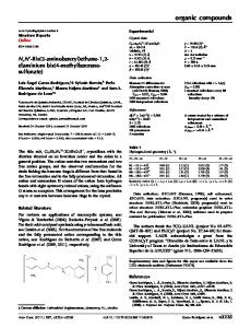
Proof. By the assumption, there exist two nonadjacent vertices u, u’ in M. Suppose there also exist two non-adjacent vertices v, v’ in N(M). Then u, u’, v and v’ form an induced 4-cycle in G, a contradiction. █ Corollary 2.2. Let G be a chordal graph containing no similar vertices. Let M be a module of G. Replace each maximal proper submodule of M by a marker vertex in the graph G[M]. Denote the resulting graph by G*[M]. Then these marker vertices are simplicial in G*[M]. If G*[M] contains at least 4 vertices, then it must be S-prime. Each such S-prime graph G*[M] is called an S- prime component of G (and is often referred to as the representative graph for M). A degenerate case is that G*[M] contains two adjacent vertices, one of which is a marker vertex. The result of an S-decomposition can be represented by a tree, where each subtree represents a nontrivial module marked by its root. For chordal graphs, a module is decomposed into its maximal submodules (these submodules are then replaced by marker vertices in G*[M] as described in Lemma 2.3). For the graph G in Figure 1 we illustrate its S-decomposition tree in Figure 2. Note that all vertices of G are represented as leaves in the decomposition tree.
G
4
7 2
6
6
7
5
8
1
5
1 4
2
3
8
3
The corresponding interval graph Figure 1. The graph G N1
1
N2
7
2
3
4
8
5
6
Figure 2. The S-decomposition tree of G The following theorem is trivially true since substituting an interval graph for a simplicial vertex in another interval graph gives rise to an interval graph. Theorem 2.3. A chordal graph G containing no similar vertices is an interval graph iff every S-prime component of G is an interval graph. The main idea of our algorithm is as follows. If the given chordal graph G is Sprime, then we try to find an interval model for G in Section 5. Otherwise, we find an
S-decomposition tree for G and find an interval model for each S-prime component of G. The algorithms for tree and model construction are all based on the construction of a special ST-subgraph of G, which is discussed in Section 3.
3. The ST-Subgraph G' and the S-Decomposition Tree In this section, we explore more properties of interval graphs that are related to the construction of S-decomposition trees. Assume the given graph G is chordal and does not have similar vertices. A vertex i is said to contain another vertex j if N[i] contains N[j]. Two adjacent vertices u, v in G are said to be strictly adjacent if none of N[u] and N[v] is contained in the other. Define the ST-subgraph G' of G to be the subgraph with vertex set V(G) whose edge set E’ consists of all those strictly adjacent pairs in G. An example of G' for the graph G in Figure 1 is shown in Figure 4. We shall construct a S-decomposition tree based on the connected components of G'. Note that, for each edge (u,v) in E-E’, we have either u contains v or v contains u. Furthermore, each simplicial vertex in G becomes an isolated vertex in G' (but not vice versa). 4
G' 6 7
2
1
5 3
8
Figure 3. The ST-subgraph G’ Define the skeleton of a module M of G to be the set of vertices in M which are not contained in any proper submodule of M. The main result of this section is Theorem 3.4, which can be proved from Lemmas 3.1 and 3.3. Let S denote the set of simplicial vertices in G. Theorem 3.4. The vertex set of each connected component of G'-S gives rise to the skeleton of a submodule of G. These connected components are called the skeleton components of G’. As an example, the components {2,7}, {5,6} in Figure 3 are the skeleton components of modules N1, N2 respectively. Lemma 3.1. Let G be a chordal graph without similar vertices. Let M be a nontrivial submodule in G. Then G'[M] is disconnected from G'[V-M] in G’. Proof. By Lemma 2.2, N(M) is a clique in G. Since every vertex in M must be adjacent to every one in N(M), there can be no strictly adjacent pairs with one vertex from M and another from V-M in G. █ Corollary 3.2. Let G be a chordal graph without similar vertices. Let M be a nontrivial submodule in G. Let GM be the graph obtained from substituting M by a marker vertex m in G. Then m is a simplicial vertex in GM. Lemma 3.3. Let G be an S-prime chordal graph without similar vertices. Let D = VS. Then G'[D] is connected.
Proof. Since G is connected, deleting a simplicial vertex does not disconnect G. Hence, G[D] must also be connected. Suppose G'[D] is disconnected. Let C, C' be two connected components of G'[D] with sizes greater than one such that there exist vertices u, u' in C, C', respectively, with (u,u') ∈ E. Since u and u’ are not strictly adjacent in G, we may assume, without loss of generality, that u' contains u in G. Hence, u' is adjacent to every vertex in N(u). We shall derive a contradiction in Claim 2. Claim 1. u' must contain every vertex in C. Proof of Claim 1. Suppose u’ does not contain a neighbor v of u in C. Then v must contain u' (since u’ cannot be strictly adjacent to v). Since v is strictly adjacent to u, there exists a vertex v' adjacent to u but not v. Since u' contains u, u' is adjacent to v', a contradiction to that v contains u'. Hence u' must contain every neighbor of u in C. Through a breadth-first-search from u in C, one can argue iteratively that u' must contain all vertices in C. █ Let Q be the set of vertices in G-C each of which is contained in some vertex in C. Claim 2. M = Q ∪ C is a nontrivial module in G. Proof of Claim 2. Let v be any vertex in G-M adjacent to a vertex u in M. We shall first argue that v must be adjacent to a vertex in C. By the definition of Q, v cannot be contained in any vertex in C. Hence, v must contain u. If u ∈ Q, then v must be adjacent to the vertex u’ in C that contains u. By the above argument, v must also contain u’. Similar to the proof of Claim1, one can argue that v must contain all vertices in C. Hence, v must contain all vertices in M; in particular, v is adjacent to all vertices in M. █ In the following we shall show how to construct the S-decomposition tree of G based on the components of G’. The containment relationships of these components can be obtained as follows. (1) Form the graph SG whose vertex set are the connected components of G’ (namely, those skeleton components of G’ as well as the simplicial vertices of G) and there exists an edge between C1 and C2 in SG iff there exist vertices u, v in C1, C2, respectively such that (u,v) ∈ E-E’. (2) Direct the edges of SG as follows. Each edge (u,v) in E-E’ connecting two components C(u) and C(v) in G’ satisfies that C(u) contains C(v) iff deg(u) > deg(v). Direct edge (C(u),C(v)) from C(u) to C(v). Thus, all edges of SG can be directed based on the degrees of the incident vertices in G. (3) The skeleton C* of the module V(G) is the only component of G’ which is not contained in some other component. Find the longest path graph (LPG) of SG emanating from the vertex representing C* (every path from C* to a node C in an LPG is the longest possible). This is exactly the Hasse diagram T(G) of the component containment relationships of G’. In Figure 4, we illustrate the Hasse diagram of the graph G’ in Figure 3. containment
4 6
skeleton component
7
2
5 simplicial vertex 3
8
Figure 4. The Hasse diagram of the containment relationships
1
Lemma 3.5. The Hasse diagram T(G) of SG satisfies the following properties: (1) T(G) is a rooted tree with root C*. (2) For each internal node C, let TC be the subtree consisting of node C and its descendants. The set of vertices of G in TC (denoted by VG(TC)) form a S submodule of G whose skeleton is C. (3) The S-decomposition tree of G can be obtained from the Hasse diagram T(G) as follows. For each internal node C of T(G), construct a node N(C) for its corresponding S-submodule VG(TC). Construct a node for each vertex in C. Let the children of N(C) be the union of the set of children of C in T(G) and the set of vertices in C. Proof. To show (1) we only have to show that the children of C* in T(G) other than the simplicial vertices of G are exactly the skeletons of maximal S-submodules of V(G). The rest can be argued by induction. By Theorem 3.4, each such child is the skeleton of an S-module of G. If such an S-module, say M1, is not maximal, then there is a maximal S-submodule of V(G), say M2, properly containing M1. This would imply that there is a path from C* through the skeleton of M2 to that of M1, longer than the direct edge from C* to the skeleton of M1, a contradiction. Since the maximal S-submodules of V(G) are disjoint, (1) follows by induction. Let M be the submodule of G whose skeleton is C. (2) follows from the fact that each vertex in M-C must be contained in some vertex in C. (3) follows by induction using Corollary 2.2. █
4. The Special Subgraph G” To find the S-decomposition tree for G it suffices to find the connected components of G’. However, discovering for every adjacent pair in G, whether they are strictly adjacent in G can be very costly. Instead, we shall show how to compute a subset E” of E' efficiently that gives rise to the same set of components of G’. A necessary and sufficient condition for a graph to be chordal is that it admits a perfect elimination ordering. This is a linear ordering of the vertices such that, for each vertex v, the neighbors of v that are ordered after v form a clique. On chordal graphs, a perfect elimination ordering can be obtained in linear time through a lexicographic breadth-first-search [11] (the resulting ordering is called a lexicographic ordering (LO)). This algorithm can be regarded as a partitioning algorithm based on a certain labeling. Imagine there is a label of n digits, initially filled with zeros, associated with each vertex. The n-th vertex is chosen arbitrarily. After the (i+1)-th vertex is chosen, put a "1" in the (n-i+1)-th digit of the labels of the neighbors of the vertex. The i-th vertex is then chosen among the unchosen vertices with the greatest label (with the first digit being the most significant digit). There are two important properties (cf. [2]) of a lexicographic ordering π. (4.1) If graph G is chordal, π -1(u) < π -1(v) < π -1(w) and (u,v), (u,w) ∈ E, then (v,w) ∈ E, namely, those neighbors of u ordered after u must form a clique. (4.2) If π -1(u) < π -1(v), then either (a) for each w with π -1(v) < π -1(w), w is adjacent to both of u, v or none of them; or (b) the largest w with π -1(v) < π 1(w) which is adjacent to exactly one of u, v must be adjacent to v. A cardinality lexicographic ordering (CLO) is an LO obtained by breaking ties in favor of the vertex with the maximal degree. Based on a CLO, Hsu and Ma [7] designed a linear time algorithm to obtain a complete S-decomposition of a chordal graph G; and by precomputing all maximal cliques of G, find a linear time recognition algorithm for interval graphs. In this paper, we use a CLO to compute a
special subgraph G” of a chordal graph G, which allows us to skip the computation of maximal cliques of G and to compute the following in linear time: (1) the S-decomposition tree of G (2) an interval model for G. Let G be a chordal graph. Perform a CLO on G. Let π denote the resulting ordering. Let S be the set of simplicial vertices in G and D = V-S. For every vertex u in D, define f(u) to be the vertex in N(u) with the smallest π-index. Since u is not simplicial, u must have a neighbor with a smaller π-index. Hence, we have π -1(f(u)) < π -1(u). Consider the subgraph G" = (V,E") whose edge set E" is obtained as follows. E" = { (u,v) | u, v ∈ D, π -1(u) < π -1(v), f(u) ∉ N(v) } Lemma 4.3. Let G be a chordal graph containing no similar vertices. Then, E" ⊆ E. Proof. This follows from the following two facts: (i) π -1(u) < π -1(v) implies N[v] ⊄ N[u] by the definition of CLO and the fact that G contains no similar vertices, (ii) f(u) ∉ N[v] implies N[u] ⊄ N[v]. █ The edge set E" can be computed in linear time as follows: for every vertex x, determine U(x) = { u | f(u) = x } (this can be done for all x through a linear scan). Now, label the neighbors of x. For every u in U(x), connect u to each (unlabeled) vertex w in N[u]\N[x] with π -1(w) > π -1(u). Three pairwise nonadjacent vertices in a graph are said to form an asteroidal triple if any two of them are connected by a path which avoids the neighborhood of the remaining vertex. Theorem 4.4 [3]. An interval graph does not contain an asteroidal triple. Theorem 4.5. If G is an interval graph, then the connected components of G” are identical to those of G’. Proof. Let u, v be two strictly adjacent vertices in G with π -1(u) < π -1(v) but (u,v) ∉ E". By the definition of E”, we must have f(u) ∈ N(v). We shall show that there exists a vertex w with π-1(v) < π -1(w) such that both (u,w) and (v,w) belong to E". This would imply that u, v are in the same connected component of G”. Since u, v are strictly adjacent, there exists a vertex t in N(u)-N[v]. By (4.1), π -1(t) < π -1(u). Since t ≠ f(u) (the latter belongs to N(v)), we have π -1(f(u)) < π -1(t) by the definition of f(u). We now have π -1(f(u)) < π -1(t) < π -1(v). Since v is adjacent to f(u) but not to t, by (4.2), there must exist a vertex ordered after v which is adjacent to t, but not f(u). Let w be such a vertex. Since (t,u), (t,w) ∈ E, we must have (u,w) ∈ E by (4.1). Similarly, since (u,v), (u,w) ∈ E, we have (v,w) ∈ E. Since (w, f(u)) ∉ E, we conclude that (u,w) ∈ E". We now show that (v,w) ∈ E". If f(v) = f(u), then by the definition of E”, we shall have (v,w) ∈ E”. If f(v) ≠ f(u), we have π -1(f(v)) < π -1(f(u)) and (f(v),u) ∉ E. Now, we must have (f(v),w) ∉ E; otherwise, since (w, f(u)) ∉ E, we must have (f(v), f(u)) ∉ E by (4.1) and we would have an asteroidal triple (t,f(u),f(v)) as shown in the subgraph of Figure 5. Hence, (v,w) ∈ E". █
f(u) edge
the CLO ordering: v
f(v), f(u), t, u, v, w f(v)
u
w
non-edge t
Figure 5. An asteroidal triple (t,f(u),f(v)) The basic scheme of our recognition algorithm is as follows. First, compute a CLO for G. If G is not chordal, stop. Otherwise, construct the subgraph G". Based on the connected components of G", compose an S-decomposition tree of G. Finally, test each S-prime component to see if it is an interval graph (Theorem 2.3). This test is the subject of the next section.
5. Constructing an Interval Model for an S-Prime Interval Graph In this section assume the graph G is an S-prime interval graph. By constructing a model for G, we mean arranging a left-to-right block sequence for G. Let S be the set of simplicial vertices in G and D = V-S. Since G is S-prime, the block sequence for vertices in D is unique. We shall directly place the intervals corresponding to the vertices into the model. The placement is divided into two stages. First, place intervals in D one by one into the model. Next place all intervals of S in one batch. In order to maintain efficiency, each interval to be placed in D is only known to be strictly adjacent to one interval in the current placement. Since we do not have information on all the strictly adjacent relationships, the order of placement is extremely important. Vertices in D will be considered according to the following ordering π': Let T be a spanning tree for G"[D]. Perform a BFS on T starting with a leaf node u1 as the root of T. Let the final ordering be π' = u1u2...u|D|. Then each ui with i > 1 has its children arranged consecutively in π'. Denote by BL(ui), the left block containing L(ui); BR(ui), the right block containing R(ui); and [BL(ui),BR(ui)] the set of block subsequence from BL(ui) to BR(ui). We place vertices of D according to the ordering π'. For the first two intervals u1 and u2 of D, let BL(u2) = {L(u1),L(u2)}, BR(u2) = {R(u1),R(u2)}. An endpoint R(uj) is said to be contained in an interval ui if BR(uj) is contained in [BL(ui), BR(ui)]. Now, place the remaining intervals {u3, ..., u|D|} of D inductively as follows. Let ui be the next interval to be placed. Let uj be the parent of ui. We first determine (uniquely) whether R(uj) or L(uj) is contained in ui using the method described in the proof of Lemma 5.1. Once this is determined, the two endpoints of ui can be uniquely inserted into the current block sequence as follows. Perform two searches starting from the block containing that endpoint of uj: one to the right of that block, the other to the left. Mark all endpoints of intervals adjacent to ui. Towards the right, find the first L-block BL* that contains an unmarked left endpoint. If BL* also contains a marked endpoint, then split B into two blocks B1, B2, where B1 contains those marked endpoints of B, and B2 contains those unmarked endpoints of B. Insert R(ui) into B1. If all endpoints of BL* are unmarked, then insert R(ui) into the Rblock immediately to the left of BL*. The insertion of L(ui) can be done symmetrically to the left. Our major result is Theorem 5.2, which can be proved based on Lemma 5.1. Theorem 5.2. The placement for vertices in D at each iteration is unique.
Lemma 5.1. Let ui be the next interval to be placed. Let uj be the parent of ui. It can be determined uniquely whether R(uj) or L(uj) is contained in ui. Proof. Let uk be the parent of uj. Assume, without loss of generality, R(uk) is contained in uj (see Figure 6). Since ui is not a child of uk, we must have (ui,uk) ∉ E”. If (ui,uk) ∉ E, then clearly, R(uj) is contained in i. If (ui,uk) ∈ E, then we shall show that L(uj) is contained in ui. Note that the test whether ui is adjacent to uk or not can be performed for all children of uj in T in time proportional to |N[uk]| + |N[uj]|. Consider the following cases: Case 1. i < j and i < k. Since (ui,uk) ∉ E”, we must have (f(ui),uk) ∈ E. Case 2. j < i and j < k. Since (f(uj),uk) ∉ E and (f(uj),ui) ∉ E, ui and uk must be on the same side, namely L(uj) is contained in both ui and uk. Case 3. k < i and k < j. Since (ui,uk) ∉ E”, we have (f(uk),ui) ∈ E. Since (uk,uj) ∈ E”, we have (f(uk),uj) ∉ E. █ uk uk uk f(u ) j
f(u i )
uj
uj
ui Case 1
ui Case 2 Figure 6. Proofs of the three cases
f(u ) k
uj
ui Case 3
Finally, all simplicial vertices of G can be placed through a left-to-right scan of the block sequence for D as follows. For each endpoint t scanned, let Q be the set of all intervals whose left endpoints have already been scanned, but whose right endpoints have not been. For each simplicial vertex u, keep a counter T(u) on the number of left-endpoints of N(u) encountered so far. Let RL(u) be the right-most left endpoint of N(u). Let LR(u) be the left-most right endpoint of N(u). Now, scan the list from left to right and update the counters Q and T(u) for each u. For each left endpoint L(v) scanned increase the counter T(·) of each simplicial vertex of N(v) by 1. As soon as the counter T(u) equals |N(u)| for a simplicial vertex u, the left endpoint currently scanned becomes RL(u). At this point, we have Q ⊃ N(u), and Q-N(u) are those intervals that are not adjacent to u whose right endpoints have not been scanned. Note that endpoints of u must be inserted between RL(u) and LR(u) at the place where the current Q-N(u) = ∅ (namely |Q| = |N(u)|). Hence, when T(u) = |N(u)| for the first time we push u into a stack. When the current Q-N(u) becomes ∅, we shall pop element from the stack until u is popped out. Note that any vertex u’ popped out the stack together with u will satisfy Q-N(u’) = ∅. If any of the above conditions is not satisfied, G is not an interval graph. Note that Q-N(u) does not have to be updated for every u at every endpoint scanning. One only has to evaluate Q-N(v) for the top vertex v of the stack at each scanning. Since there may be independent simplicial vertices with the same neighbors, the interval orders among them can be arbitrary. Since all of the above placement can be carried out uniquely (up to the permutation of independent simplicial vertices with the same neighborhood), if any discrepancy occurs, we can immediately conclude that the given graph is not an interval graph; otherwise, an interval model is constructed whose overlapping relationship can be checked against the adjacent relationship of G.
6. Complexity Analysis
The algorithm involves the following steps each of which can be done in O(m + n) time. (1) The construction of CLO in Section 4. (2) The construction of the special subgraph G” in Section 4. This provides the basis for the construction of the decomposition tree as well as the interval models. (3) The construction of the Hasse diagram for containment relationship of components in G” (this involves the computation of a longest path graph) in Section 4. (4) The construction of the S-decomposition tree from the Hasse diagram in Section 4. (5) The construction of interval models for each S-prime component of G in Section 5. Hence, the total running time of the recognition algorithm is linear. Since a by-product of this algorithm is an (unique) S-decomposition tree, and each prime component almost has a unique interval model, it would not be difficult to derive a linear time isomorphism algorithm for interval graphs from this recognition algorithm. We should note that a linear time isomorphism algorithm was designed in [9] based on labeled PQ-tree.
7. On-Line Construction of the S-Decomposition Tree Below, we assume that the given graph G is indeed an interval graph. If this is not the case, some violation would be discovered along the way and one could then terminate the recognition algorithm. We shall apply the vertex partitioning strategy described below to construct the current decomposition tree efficiently. At each iteration we need to keep the block sequence for the representative graph of each prime component. This sequence is stored as a linked list. For each vertex in G we record the blocks containing its two endpoints.
Theorem 7.1. At each iteration (when a new vertex v is added), the S-decomposition tree can be updated in O(deg(v)) time.
This theorem can be proved by following through the construction procedure described below. Initially, the decomposition tree is empty. Let T be the current tree associated with the current graph G. Let v be the new vertex added to G. Mark all vertices of G that are adjacent to v. The nodes of T can be classified as follows. 1. A node of T is said to be full if every vertex in its corresponding submodule is adjacent to v. 2. A node is said to be partial if some but not all vertices in its corresponding submodule are adjacent to v. 3. A node is said to be empty if no vertex in the submodule it represents is adjacent to v. A leaf node of T is either full or empty. Note that it suffices to mark the neighbors of v in G to identify all the partial and full nodes in a bottom up fashion. Hence the
number of steps involved in the labeling will be proportional to deg(v). The ancestors of a partial node must all be partial. Two intervals are said to cross each other if they overlap but none is contained in the other. A submodule M is said to cross the interval v and vice versa if (i) v overlaps with some but not all intervals in M; and (ii) v overlaps with some interval u (outside M) which does not overlap with any interval in M. A submodule M is said to be contained in v if every interval in M overlaps with v. A module M is said to contain v if (i) v overlaps with some interval in M; and (ii) for any u in G\M, v overlaps u iff every interval in M overlaps with u. The construction of the S-decomposition tree for G ∪ {v} is done recursively in a top-down fashion starting with the root module. At each partial submodule, we illustrate how to insert the endpoints of v into the block sequence of the representative graph of the submodule. The root module M(G) must contain v. We shall first describe the change of the block structure in case both endpoints of v are inserted into the same component M. Consider the representative graph for M and its corresponding block sequence. Consider the following cases: 1. M is a type I module (a clique): split the node for M into two nodes representing two submodules M1 and M2 with M1 ∪ M2 = M, where M1 consists of all vertices of M that are adjacent to v and M2 = M - M1. Connect these two nodes to the parent of the node for M. Connect all vertices in M1 to the node for M1 and those in M2 to the node for M2. Construct a node for v and connect it to M1. Construct a new node for v and connect this node to that for M1. This is illustrated in Figure 7. parent of M
parent of M
M
M1
M2
v Figure 7. The split of a type I module
2. M is a type II module: Let BL be the block containing the right-most left endpoint of neighbors of v and BR the block containing the left-most right endpoint of neighbors of v. Consider two subcases: (1) v is a simplicial vertex: BL should be to the left of BR. Thus, the endpoints of this new interval v should be inserted into a new block located in between BL and BR. The exact way to locate the position of this block will be described in Section 4. Consider the following three subcases: (a) v has a true twin, say v', in the representative graph: then a type I node consisting of {v,v'} is created. We then replace the node for v' in M by this node and connect the nodes for v and v' to this new node. (b) v has a false twin, say v', in the representative graph: then a type II node consisting of {v,v'} is created. We then replace the node for v' in M by this node and connect the nodes for v and v' to this new node.
(c) v has neither a true twin nor a false twin: then v is not contained in any nontrivial submodule of M ∪ {v}. Thus, we construct a new node for v and connect this node to the node for M. (2) v is not a simplicial vertex: BR should be to the left of BL. The left endpoint of v should split BR and the right endpoint of v should split BL. In this case v cannot have a false twin. Consider the following subcases: (a) v has a true twin, say v', in the representative graph (with endpoints in the same left and right block as v does): then a type I node consisting of {v,v'} is created. We then replace the node for v' in M by this node and connect the nodes for v and v' to this new node. (b) v does not have a true twin: then v is not contained in any nontrivial submodule of M ∪ {v}. Thus, we construct a new node for v and connect this node to the node for M. Recursively insert the endpoints of v into any submodule of M crossing v. Next, we consider the case that v crosses a module M and only one endpoint of v is inserted into the block sequence for the representative graph of M. Without loss of generality, assume we are inserting the left endpoint of v. Note that in this case the node for v has already been connected to higher level nodes, so vertex v only split the lower level submodules. Consider the following cases: 1. M is a type I module (a clique): this case is analogous to the above. 2. M is a type II module: let BR be the block containing the left-most right endpoint of neighbors of v. Then the left endpoint of v should split BR. The new block sequence will then be merged with the one containing the right endpoint of v. Note that in the above operations, if it is found that some parent has only one child then this parent can be deleted and replaced by this child. We illustrate an example of our algorithm below. Suppose we add another vertex 10 to the graph G with neighbors 2, 7 and 9 (call the resulting graph G1). We first insert both endpoints of v into the root module N1 using case 2(2)(b). Since v crosses the submodule P, we insert the left endpoint of v into the submodule P using case 3(2). Since v crosses the submodule S, we insert the left endpoint into the submodule S using case 1.
8. Updating the Queue of Cut Widths In addition to computing the block sequence for each prime component, we also construct a priority queue of cut widths. We illustrate the queues for the graph G in Figure 9.
The block sequences for G are (a) the sequence for N 1is {7,P},{P'},{2,},{7'},{1},{1',2'} (b) the sequence for N is {4,6},{4'},{5},{6'},{3},{3',5'} 2 The queues of cut widths are the same for both components 1 1 1
2
1
1
2
1
2
Figure 9. The queues of cut widths for the components of G
The main reason for keeping track of this queue is that they can be used more effectively for interval graph test. This can be explained as follows. Supposing the newly added vertex v is simplicial (namely, its neighbors form a clique) in some prime component H. Denote the current unique interval model of the representative graph for H by D. To test whether H and v form a new interval graph, we need to check whether it is possible to insert the interval for v into model D. By the discussion in Section 3, both endpoints of v should be inserted into new blocks created in between the blocks BL and BR. Since it is quite likely that intervals in HN[v] form a barrier preventing the inclusion of v, it might appear that we need to check vertices not in N[v], which could become quite inefficient. Consider for example, the interval model in Figure 10. Supposing we are adding a new interval v which overlaps only with intervals {1,2,3,4}. Thus, we need to locate the place for the new blocks containing the endpoints of v. However, without additional information, it seems that a search involving vertices not adjacent to v is unavoidable.
Inserting a new interval which only overlaps with intervals 1, 2, 3 and 4
1 2 3 4 5
8 6
9 10
7
the right cut Figure 10. Finding the right cut for the simplicial vertex We resolve this problem by maintaining a concatenable queue of cut widths in D and checking whether the minimum cut width of D within the two blocks BL and BR equals |N(v) ∩ H|. Once this cut width is found one can quickly identify the location of the cut by tracing down the queue and update it. In general, we shall associate a queue of cut widths for each prime component of the graph in addition to the block sequence. Whenever a new interval is inserted we first determine the new decomposition tree as described in the last section and the change of the block sequences. Then we need to specify the change of the associated queues. We first locate the two blocks BL and BR. If the new vertex v is a simplicial vertex, we use the queues to determine the location of the new blocks. Otherwise, the endpoints of v should split BL and BR, we can perform the normal tree spliting to update the queue. Next, we discuss an efficient method for updating the queue when several prime components are combined into a new component M ∪ {v} = Mv , where M is the smallest submodule of G containing v. The queue update is done iteratively in a topdown fashion, starting from the module M. We first determine the unique way to insert the endpoints of v into the block sequence of M in a manner described above. For any submodule, say M', split by v (there can be at most two of these) we repeat the above process with M' and so on. The final queue and block sequence for Mv is obtained by recursively substituting the new queues and block sequences of the submodules back to its immediate supermodules. Now consider the cut widths associated with Mv. Along the path from a submodule M' to M, every intermediate submodule represents a simplicial vertex in the representative graph of its parent module. To update the cut width for the queue
of Mv, we can precompute the cut width increment for every block in these components and determine the final cut width all at once. Initially, we simply concatenate the individual queues of neighboring node in the path using the current cut widths associated with the nodes. Each concatenation takes at most O(log n) time, the total number of concatenations equals the number of partial nodes in T. Since the total number of nodes ever created for the decomposition tree is at most O(n) the total concatenation time is at most O(nlog n). If the above algorithm terminates without encountering any contradiction, then we conclude that the current graph is an interval graph; otherwise, it is not. Below, we illustrate the corresponding change of the priority queue for the cut widths of N2 in Figure 11. 1 1
1 1
2
2 2
1
3
2
2
3
2
2
3
1
2
1
2
Figure 11. The cut width queue of N1
References
1. K. S. Booth and G. S. Lueker , Linear algorithms to recognize interval graphs and test for the consecutive ones property, Proc. 7th ACM Symp. Theory of Computing, (1975), 255-265. 2. K. S. Booth and G. S. Lueker, Testing for the consecutive ones property, interval graphs and graph planarity using PQ-tree algorithms, J. Comput. Syst. Sci. 13, (1976), 335-379. 3. D. R. Fulkerson and O. A. Gross, Incidence Matrices and Interval Graphs, Pacific J. Math. 15, (1965), 835-855. 4. M. C. Golumbic, Algorithmic Graph Theory and Perfect Graphs, Academic Press, New York, 1980. 5. W. L. Hsu , O(mn) Recognition and Isomorphism Algorithms for Circular-Arc Graphs, SIAM J. Comput. 24, (1995), 411-439. 6. W. L. Hsu and C. H. Ma, Fast and Simple Algorithms for Recognizing Chordal Comparability Graphs and Interval Graphs, Lecture Notes in Computer Science 557, 52-60, (1991), to appear in SIAM J. Comput. 7. W. L. Hsu, A simple test for interval graphs, Lecture Notes in Computer Science 657, (1992), 11-16.
8. N. Korte and R. H. M ö hring, An incremental linear time algorithm for recognizing interval graphs, SIAM J. Comput. 18, (1989), 68-81. 9. G. S. Lueker and K. S. Booth, Interval graph isomorphism, JACM 26, (1979), 195. 10. J. Spinrad, On Comparability and Permutation Graphs, SIAM J. Comput. 14 (1985), 658-670.