AN OPEN-SOURCE GPU-ACCELERATED FEATURE EXTRACTION ...

AN OPEN-SOURCE GPU-ACCELERATED FEATURE EXTRACTION TOOL Josef Mich´alek and Jan Vanˇek Department of Cybernetics and New Technologies for the Information Society University of West Bohemia, Plzen, Czech Republic [email protected], [email protected] ABSTRACT

2. HIGH PERFORMANCE GPU IMPLEMENTATION

An extraction of feature-vectors from speech audio signal is a computationally intensive task. However, MFCC and PLP features remain the most popular for more than a decade. We made a GPU-accelerated implementation of the feature extraction processing. The implementation produces identical features as the reference Hidden Markov Toolkit (HTK) but in a fraction of the elapsed time. The saved time can be invested elsewhere and thus it can speed-up research. The implementation was developed in CUDA which supports NVidia GPUs only. So, we added an Open-CL implementation to support any current GPU. The project is an open-source package, thus research community can modify or adapt the implementation to their needs.

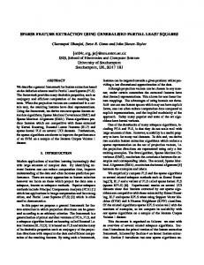
The general purpose GPU programming is very specific. A programmer should perfectly understand the programming model and GPU hardware abilities. Following of the optimization guides is necessary [8], [9]. However, it is often not enough to get the high-performance implementation. An algorithm can be implemented in various ways, but only a few of them achieve a high performance. In this section, we have described the implementation that gives the best performance. The individual algorithm steps are illustrated on Figure 1.

1. INTRODUCTION GPU devices are highly parallel multi-core systems allowing an efficient processing of large blocks of data. A using of GPU-acceleration of numerically intensive algorithms becomes popular because GPUs power and energy efficiency grow fast in contrast with CPUs. Currently, an open GPU computing platform - OpenCL - is supported by all GPU vendors [1]. However, Nvidia CUDA platform is still popular for its debugging and profiling ability, and available libraries [2]. The GPU-acceleration was successfully applied in the speech processing field also. An algorithm to evaluate acoustic model probabilities was presented in [3]. Even an entire GPU-accelerated speech recognition system was described in [4]. GPU FFT libraries from many sources are also available and they can make a base of the feature processing [5], [6]. Our implementation is focused on an off-line processing of very large data sets. With off-line constrains, all the optimization techniques can be utilized and the final performance is better. The implementation details are described in the next Section 2. The last Section 3 shows elapsed times for various scenarios in comparison with the well-known speechprocessing standard - HTK [7] and with a popular open source tool openSmile [10].

2.1. MFCC 2.1.1. Segmentation The first step of MFCC calculation is a dividing samples into frames and an applying window function on each frame. Frames overlap each other, so simple memory copy cannot be used. Two approaches were tested: 1. Copying each frame separately from the host memory to the correct position in the device memory. 2. Copying all input data into a temporary buffer in the device memory and executing a custom kernel to segment data into the frames. The second approach turned out to be faster. Even though, it copies each frame twice. Only one memory transaction between host and device is the key difference. The frame length is rounded up to the closest power of 2 and padded with zeros for faster processing of the next steps of the MFCC calculation. The kernel that segments data into the frames was also modified to apply a window function on each frame. The window function values are stored in the global device memory and copied to the fast shared on-chip device memory at the beginning of the kernel. This eliminates redundant reads from the global memory and speeds up execution. 2.1.2. Fourier Transform

This research was supported by the Grant Agency of the Czech Republic, ˇ GBP103/12/G084. project No. GACR

Next step is calculating the power spectrum of each frame.

Input Segmentation

DCT

FFT

Delta

Transposition

Normalization

Mel filters

Output

(a) MFCC

Input Segmentation

LPC

FFT

Cepstrum

Transposition

Delta

Filters

Normalization Output (b) PLP

Fig. 1. Block diagram of implemented methods The Fourier transform is calculated using CUFFT library and its implementation of the FFT algorithm in the CUDA variant. The AMD FFT implementation is used in the OpenCL case. These libraries use several optimizations and the performance peak is obtained if the length of input data is power of 2. For a real input of length N , CUFFT returns complex data of length N/2 + 1. The rest of the Fourier coefficients can be calculated from these. Because only magnitude is needed, sign of imaginary part of coefficients is not important and a code branching can be avoided. A custom kernel was written to calculate the magnitude of the complex Fourier coefficients. This power spectrum is then stored into the device memory in transposed order which enables a fast coalesced access in the mel-filter-bank kernel. 2.1.3. Mel Filter Bank Applying the mel-filter-bank means calculating discrete convolution of the filter function and the power spectrum for each filter. This operation can be easily implemented using matrix

multiplication, where rows of the left matrix are input frames and columns of the right matrix contain the filter function values for the individual filters. Because the majority of such filter matrix is filled with zeros, this approach leads to waste memory throughput, where zeros are read and written, and also redundant instructions. To omit the junk computations and memory transfers, we wrote an optimized kernel to apply mel-filter-bank. Each frame is processed by one thread. Threads read the input data in order from the first to the last one, multiply the data by the filter function value and add the result to a register. When the end of the filter is reached, the accumulated value in the register is equal to value of the particular mel-filter. Logarithm of this value is then written into an output buffer. Because only two filters overlap at one point, only two registers are needed for this calculation. The filter function values are stored in a matrix, which is generated during program initialization. Data is stored in the device memory frame by frame and it would lead to slow uncoalesced access in this kernel. From that reason, the power spectrum is transposed before the melfilter-bank kernel is executed.

2.1.4. DCT The last step in the MFCC calculation is decorrelation. Our implementation uses type-II DCT. A matrix of the DCT coefficients is constructed during the program initialization and DCT of every frame is calculated by multiplying all data by the DCT matrix. The matrix multiplication is done using CUBLAS library or AMD OpenCL library. These libraries allow to specify if each matrix should be read transposed or not. For our input data, the multiplication was the fastest if both matrices were transposed. Transposing output of the mel-filter-bank kernel also ensures coalesced writes to memory.

2.1.5. Delta Coefficients Delta coefficients for one frame are computed from its several neighboring frames. It means, that the input data must be read several times to calculate the delta coefficients. Since the input data are in the global memory, the read operation can be costly and it should be avoided if possible. Our implementation calculates the delta coefficients in blocks with a predefined size. The block of the input data is copied into shared memory and all subsequent calculations on this block use only data in the shared memory and not in the global memory. Only the overlapping block boundaries data which are needed to calculate the delta coefficients are read twice. Acceleration (delta-delta) coefficients are calculated using the same kernel, only executed on the delta coefficients.

2.1.6. Normalization Our implementation supports several normalization types. Data characteristics, like mean or variance, must be gathered prior to normalization itself for some of them. The solution using two kernels turned out to be the fastest one. Input data are divided into specific number of blocks and the first kernel gathers characteristics for such blocks. The first kernel results are then merged by the second kernel. Another kernel is then executed to do the normalization itself. It copies required data characteristics to the shared memory to minimize global memory reads and performs an in-place normalization. 2.2. PLP PLP speech analysis consists of several parts. Some of them are identical to MFCC. Segmentation, Fourier transform, delta coefficients and normalization is implemented the same way as in the MFCC case. PLP uses power spectrum squared right after FFT that is only an exception. 2.2.1. Filter Bank Filters used in PLP have different shape than those used in MFCC, but filtration itself is done the same way. Many filters overlap at one point, so the same approach as in mel-filtering cannot be used. Filters are stored in a matrix, where each row represents particular filters. We wrote a kernel that multiplies the input data by this filter matrix. Because filters occupy only minor portion of the matrix, special care is taken to loop only over significant values during the matrix multiplication. After the filter value is calculated, it is raised by the exponent of 0.3 and written into the output buffer.

they are flushed into the global memory at the end of calculations only. An all-pole model order is usually small enough to fit all linear prediction coefficients into the shared memory. If there is not enough space, a fallback kernel is executed, which operates only with the global memory. 2.2.3. Cepstral Coefficients Cepstral coefficients represent the output of our implementation. They are calculated from linear prediction coefficients using another recursive algorithm. The same approach as in the LPC calculation was chosen, where all the output data resides in the shared memory as long as possible and they are flushed into the global memory when they are not needed anymore. 3. RESULTS 3.1. Experiment Setup HTK was chosen as a reference implementation of MFCC and PLP. The same setup was used also for openSMILE (marked as oS in tables bellow). The feature processing implementation was tested on several data sets, each 10 hours long. Input data was sampled at 8 kHz and 44 kHz to show processing performance on the two common sample rates, telephone and audio CD quality. Tests were also run on input sound files of variable length. We select two categories. Lengths between 10-20 seconds are marked as short files and 5-10 minutes for long files. All tests were performed on system with following configuration: • CPU: Intel Core 2 Quad Q6600 • Motherboard: Asus P5Q-E

2.2.2. LPC

• GPU: NVidia GTX 660

To calculate linear prediction coefficients, one musts get autocorrelation coefficients firstly. These can be calculated as a linear combination of the filter values from the last step. In our implementation, this is done using CUBLAS or AMD library. A matrix is constructed during the program initialization and the filter values are multiplied by the matrix. The result of this operation is a matrix of autocorrelation coefficients with each row corresponding to the particular frame. Then, we can apply Levinson-Durbin algorithm to calculate linear prediction coefficients. This algorithm is recursive and cannot be easily parallelized. Therefore, each frame is processed by one thread. Input data is organized in such a way, that the coalesced access occurs as often as possible and threads in warps do not diverge. Algorithm uses some output data to calculate other output data and this leads to too many global memory accesses. Therefore, all output data is saved into the shared memory and

• SSD: Samsung SSD 830 256 GB • HDD: Seagate Barracuda ST2000DM001 The same input and output drive is used for test setups HDD to HDD and SSD to SSD. Storage device speed was also limited due to motherboard supporting only SATA II. MFCC configuration details: • Window size: 20 ms • Window overlap: 10 ms • Filter count: 15 for 8 kHz, 25 for 44 kHz • Output cepstral coefficients: 13 including 0’th • Delta and acceleration window size: 3 PLP configuration details:

Table 1. MFCC parameterization time in seconds HDD → HDD Input Short 8 kHz Long 8 kHz Short 44 kHz Long 44 kHz

SSD → SSD

SSD → HDD

HDD → SSD

HTK

oS

Afet

HTK

oS

Afet

HTK

oS

Afet

HTK

oS

Afet

143.2 109.3 364.6 272.2

347.3 282.9 998.2 875.7

37.5 6.1 172.3 46.8

109.2 88.6 273.8 252.6

346.4 281.9 1002.5 875.1

28.6 6.0 57.1 28.9

61.1 88.6 275.3 254.2

346.5 283.4 997.1 874.2

33.9 6.5 63.1 28.4

137.1 97.5 336.7 266.6

344.6 283.2 1001.0 873.9

29.7 6.1 109.1 37.9

Table 2. PLP parameterization time in seconds HDD → HDD Input Short 8 kHz Long 8 kHz Short 44 kHz Long 44 kHz

SSD → SSD

SSD → HDD

HDD → SSD

HTK

oS

Afet

HTK

oS

Afet

HTK

oS

Afet

HTK

oS

Afet

108.2 82.8 298.8 201.5

361.5 293.8 1008.9 889.6

36.6 7.1 175.7 49.5

76.1 59.8 200.0 183.0

363.3 299.0 1012.7 893.1

29.9 7.3 62.0 31.7

43.5 59.1 202.7 183.6

360.4 289.4 1007.1 886.9

34.6 7.3 70.3 31.0

101.6 68.1 255.5 198.6

358.6 289.5 1008.2 888.0

30.4 7.0 120.3 40.5

Segmentation

Data processing

Normalization

6.8%

15.0% 26.4%

26.9%

Delta coef. (3.8%)

93.2%

DCT (3.5%)

6.9% 17.5% FFT

Mel filter bank Transposition

Other (a) Application overview

(b) Data processing

Fig. 2. Time spent in various program sections for MFCC (Long 8kHz, from HDD to HDD) Data processing

Segmentation

9.6%

11.5%

Normalization 17.0%

Delta coef. (2.8%)

FFT

Cepstral coef. (3.3%)

19.0% 9.6% 90.4%

LPC 12.0%

24.9%

Transposition Other (a) Application overview

Filter bank (b) Data processing

Fig. 3. Time spent in various program sections for PLP (Long 8kHz, from HDD to HDD)

• Window size: 20 ms • Window overlap: 10 ms • Filter count: 15 for 8 kHz, 25 for 44 kHz plus 2 border filters • All-pole model order: 12 • Output cepstral coefficients: 13 including 0’th • Delta and acceleration window size: 3 Output features were normalized to zero mean, matching Z in HTK’s parameter TARGETKIND. Duration of program execution was measured and all the measured times are shown in Table 1 for MFCC and in Table 2 for PLP. Only a small part of application elapsed time belongs to the data processing, as shown in Figures 2a and 3a. The rest of the elapsed time consists of the GPU device initialization, including initialization of program memory structures, and mainly disk I/O. Figures 2b and 3b show portions of time spent in each part of implemented speech analysis methods. The most of elapsed time is spent in disk I/O operations. It illustrates a large difference between short and long files scenarios as well as the pie charts. Therefore, using of SSD drives are recommended for the data processing. Even if the data processing represents only a fraction of the total time, the total speed-up is substantial. The speed-up varies between 3times and 18-times and it is dependent on the scenario. The largest difference is in the Long 8kHz scenario. The total processing performance varies between 0.00017 and 0.005 RTF. 4. CONCLUSION The GPU-accelerated high-performance implementation of MFCC and PLP features was described in this paper. The implementation produces identical features as the reference Hidden Markov Toolkit (HTK) but in a fraction of the elapsed time even though the most of the elapsed time is spent on I/O disk operations. A large set of tests was performed with 10 hours of audio data. The total speed-up varies between 3-times up to 18-times and even more with comparison to slower openSMILE. In the best case, the 10 hours long audio database was processed in 6 seconds. The project is an open-source package, thus research community can use it freely. Also, one can modifies or adapts the implementation. The project is available at http://sourceforge.net/ projects/accelfeatextr/. 5. REFERENCES [1] Khronos Group Std.: The OpenCL specification, version 1.1. http://www.khronos.org/registry/cl/ specs/opencl-1.1.pdf

[2] NVIDIA corp.: CUDA: NVIDIAs parallel computing architecture. http://www.nvidia.co.uk/ object/what_is_cuda_new_uk.html [3] Vanek J., Trmal, J., Psutka, J.V., Psutka, J.: Optimized Acoustic Likelihoods Computation for NVIDIA and ATI/AMD Graphics Processors. IEEE Transactions on Audio, Speech and Language Processing, Vol. 20, 6, pp. 1818-1828, 2012. [4] Chong J., Gonina E., Yi Y., Keutzer K.: A Fully Data Parallel WFST-Based Large Vocabulary Continuous Speech Recognition on a Graphics Processing Unit. In Proc. of INTERSPEECH 2009, Brighton, United Kingdom. [5] Moreland K., Angel E.: The FFT on a GPU. In Proc. of SIGGRAPH/Eurographics Workshop on Graphics Hardware 2003 Proceedings, July 2003, pp. 112119. [6] Govindaraju N., Lloyd B., Dotsenko Y., Smith B., Manferdelli J.: High performance discrete Fourier transforms on graphics processors. In Proc. ACM/IEEE conference on Supercomputing 2008. [7] S. Young et al.: The HTK Book (for HTK Version 3.4), Cambridge, 2006. [8] NVIDIA corp.: The CUDA C best practices guide, version 3.2. NVIDIA http://developer. download.nvidia.com/compute/cuda/ 3_2_prod/toolkit/docs/CUDA_C_Best_ Practices_Guide.pdf [9] AMD Company: AMD Accelerated Parallel Processing, OpenCL Programming Guide. http://developer. amd.com/gpu [10] Florian Eyben, Martin Wllmer, Bjrn Schuller: openSMILE - The Munich Versatile and Fast Open-Source Audio Feature Extractor. Proc. ACM Multimedia (MM), ACM, Florence, Italy, ISBN 978-1-60558-933-6, pp. 1459-1462, 25.-29.10.2010.