Feature Extraction Using Genetic Algorithms

Feature Extraction Using Genetic Algorithms M. Pei1, E. D. Goodman1, W. F. Punch2 1

Case Center for Computer-Aided Engineering and Manufacturing 2

Department of Computer Science Genetic Algorithms Research and Applications Group (GARAGe) Michigan State University, 2325 Engineering Building, East Lansing, MI 48824 e-mail: [email protected]

Abstract. This paper summarizes our research on feature selection and extraction from high-dimensionality data sets using genetic algorithms. We have developed a GA-based approach utilizing a feedback linkage between feature evaluation and classification. That is, we carry out feature selection or feature extraction simultaneously with classifier design, through “genetic learning and evolution.” This approach combines a GA with a classifier system. The classifier can be a standard K-Nearest-Neighbor decision rule, a production rule or another classifier. Here we use a K-Nearest-Neighbor classifier as an example to introduce this general method. We apply this approach on a series of artificial test data and on real-world biological data to show the utility of this approach.

1 Introduction The growing glut of data in the worlds of science, business and government create an urgent need for a new generation of automated and intelligent tools and techniques which can analyze, summarize, and extract “knowledge” from raw data [1]. Most knowledge discovery or data mining tools and techniques are based on statistics, machine learning, pattern recognition or artificial neural networks. The great challenge for data mining comes from huge databases of noisy, high-dimensionality data. Genetic algorithms (GAs) are good candidates for attacking this challenge since GAs are very useful for extracting patterns in multiclass, high-dimensionality problems where heuristic knowledge is sparse or incomplete [2] [3]. The data mining approach normally includes the three major steps in the knowledge discovery process: selection, cleaning, transformation and projection of data; mining the data to extract patterns; and evaluating and interpreting the results. The first step is data preprocessing, which is important before any learning or discovery algorithms of data mining are carried out. The key operation of data preprocessing is feature selection and extraction. Mining is only one step in the overall process. The quality of mined information depends not only on the effectiveness of the data mining technique used, but also on the quality and quantity of the data preprocessed. All of these steps are usually treated as independent on the path from data to knowledge, but any one step can result in changes in preceding or succeeding steps, often requiring starting from scratch with new choices and settings.

In this paper, we take classification as the main data mining task to show the general model of our approach. The data mining approach we have developed is based on a genetic algorithm which combines the preprocessing step of feature selection and extraction and the classification step into an automated loop. In a decision-theoretic or statistical approach to pattern recognition, the classification or description of data is based on the set of data features used. Therefore, feature selection and extraction are crucial in optimizing performance, and strongly affect classifier design. Defining appropriate features often requires interaction with experts in the application area. In practice, there is much noise and redundancy in most highdimensionality, complex patterns. Therefore, it is sometimes difficult even for experts to determine a minimum or optimum feature set. The “curse of dimensionality” becomes an annoying phenomenon in statistical pattern recognition, artificial neural network and other data-mining learning techniques. Researchers have discovered that many learning procedures lack the property of “scalability” -- i.e., these procedures either fail or produce unsatisfactory results when applied to problems of larger size[6] [7] [8]. To address this scalability problem, we present an approach for automatic feature selection and extraction using genetic algorithms (GA’s). The basic operation of this approach utilizes a feedback linkage between feature evaluation and classification. That is, we carry out feature transformation and classifier design simultaneously, through “genetic learning and evolution.” The objective of this approach is to find a reduced subset among the original N features such that useful class discriminatory information is included and redundant class information and/or noise is excluded. We take the following general approach. The data’s original feature space is transformed into a new feature space with fewer features that (potentially) offer better separation of the pattern classes, which, in turn, improves the performance of the decision-making classifier. The criterion for optimality of the feature subset selected is usually the probability of misclassification. Since the number of different subsets of N available features can be very large, exhaustive search is computationally infeasible and other methods must be examined. In the field of pattern recognition, a number of heuristic techniques have been used, but it is not clear under what circumstances any one heuristic should be applied, as each has its good and bad points. In order to apply a GA to classification/discrimination tasks and work out feature transformations, we combine the GA with a K Nearest Neighbor decision rule, calling the result the GA/KNN hybrid approach. Here the GA defines a population of weight vectors w*, where the dimension of each w* is the dimension of the data pattern x for each example. Each w* from the GA is multiplied with every sample’s data pattern vector x, yielding a new feature vector y for the given data. The KNN algorithm then classifies the entire y-transformed data set. The results of the classification for a known “training” sample set are fed back as part of the fitness function, to guide the genetic learning/search for the best transformation. The GA result is the “best” vector w* under the (potentially conflicting) constraints of the evaluation function. For example, the “best” w* might be both parsimonious (have the fewest features) and give the fewest misclassifications. Thus, the GA searches for an optimal transformation from the original pattern space to feature space for improving the performance of the KNN clas-

sifier[3]. In the following sections, we describe the basic concepts of our approach; present the GA/KNN approach in more detail; show the results of several experiments; then finally propose some brief conclusions and offer areas of future study.

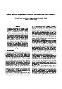
2 GA/KNN Hybrid Approach 2.1 Basic Concept of the Approach In the design of automatic pattern classifiers, ideally the problem of feature selection and extraction on the one hand and the classifier design on the other should not be considered independently. Yet, for practical considerations, most researchers make the simplifying assumption that the feature selection/extraction stage and the classification stage are independent. However the ultimate goal is correct classification with a corresponding feature pattern extracted and the intermediate step of feature extraction and dimensionality reduction is, in a sense, subservient to that goal and is not an end in itself. It would be better to couple feature selection/extraction with effective classification techniques[4]. This implies some sort of classification decision feedback mechanism to modify or adapt the feature extractor. Our research follows this direction. The approach which adopt the above idea is a supervised induction, i.e. “genetic learning and evolution,” as shown in Figure 1. N=Finite dimensional

K = number of classes Feature Extractor

Pattern Space

Classifier Feature Space Genetic learning and Evolution

Classification Space

Feedback

Figure 1. Feature Extractor and Classifier with Feedback Learning System In the GA/KNN hybrid approach, as mentioned above, a genetic algorithm using a K Nearest Neighbor decision rule searches for a “best” diagonal matrix [W] or weight vector w* -- i.e., a “best” transformation from pattern space to feature space for improving the performance of the KNN classifier [3] -- under potentially conflicting constraints of the evaluation function. The whole structure of the GA/KNN hybrid approach is shown in Figure 2. 2.2 Different Transformations Using a GA Based on the above discussion of a GA approach to feature extraction, we formally

describe the problem by defining the mapping function M() and criterion function J().

. Initialize Population (random set of weights w*) New Population

Training x data set

y = M(x) = W x Evaluate by KNN Rule

Yes

Satisfy?

No GA

Evolution Selection Crossover

Best set of weights w*

Mutation

Figure 2. The structure of GA/KNN approach We define w*, the weight vector, to be a N = |x| vector (or NxN diagonal matrix [W]) generated by the GA, to multiply each pattern vector x, yielding the new feature vector y. That is, (1) linear transformation y = M(x) = Wx where

...˙ 0 0 w 2 ... 0 . . . . . , or w* = [w1,w2, …, wΝ], . . . . .

w1 0 W =

x = [x1, x2, ⋅ ⋅ ⋅ , xN]

0 0 0 0 wN

• wi ∈{0,1}, 1≤ i ≤Ν. When we use only binary values for w*, we interpret it as follows: if the ith weight

component is one, then the ith feature is preserved in feature space; otherwise, the feature is discarded from the feature set. Thus we perform feature selection to define an optimal subset and (potentially) reduce the dimensionality of the original data pattern[5]. • wi ∈[a, b], such that wi ∈[0.0, 10.0] 1≤ i ≤Ν. We can instead do feature extraction by allowing the values of the weight components to range over some values [a, b], such as 0.0 to 10.0 (presuming that the features are first “normalized” to some standard range). That amounts to searching for a relative weighting of features that gives optimal performance on classification of the known samples. Thus we are selecting for features in a linearly transformed space. Those weight components that move towards 0 indicate that their corresponding features are not important for the discrimination task. Essentially, those features “drop out” of the feature space and are not considered. Any feature that moves towards the maximum weight indicates that the classification process is sensitive to changes in that feature. That feature’s dimension is elongated, which probably reflects that an increased separation between the classes gave better resolution. The resulting weights indicate the usefulness of a particular feature, sometimes called its discriminatory power.[4][8] Usually, only feature selection can reduce the overall cost of measurement acquisition, since feature extraction utilizes all information in the pattern representation vector x to yield feature vector y of lower dimension. But in the case above, the simple diagonal transformation certainly can reduce the cost of measurement. (2) nonlinear transformation, as, for example: y = M(x) = Wx* where

x* = [x1, x2, ⋅ ⋅ ⋅ , xN, (xi•xj)1, (xn•xm)2, ⋅ ⋅ ⋅ , (xr•xs)k], for example, ˙ 0 ... 0 w 2 ... 0 . . . . . 0 . . . . 0. 0

w1 0 W =

, or

w* = [w1,w2, …, wΝ, wN+1, …, wN+k ],

0 0 0 0 wN + k

The previous linear transformation can mainly be used on data patterns with classes which are linearly separable based on scaling or other linear operations. However, linear transformations are not necessarily sufficient for effective feature selection and extraction, so an extended form of the above linear transformation is used here. We have investigated the use of nonlinear transformations to address the feature extraction and subsequent classification of data patterns, where those data patterns have correlations between different feature fields. This approach is based on an a priori knowledge of possible forms of the relationship of the features and the use of a GA to discover which of those forms best captures the relationship.

The various combinations (xi•xj)1, (xn•xm)2, ⋅ ⋅ ⋅ , (xr•xs)k in x* form a set of new features which can be constructed and discovered by performing various mathematical or logical operations. Choice of appropriate combinations is obviously problem dependent. In our experiments, we tested an example data pattern which consists of 15 features, any feature of which by itself is not discriminatory but which does contain two combinations of features which are discriminatory. The search problem is NP hard[5]. Originally, for even moderate numbers of features (say between 15 and 30) the problem must be solved with the aid of suboptimal heuristic methods. These methods, by definition, do not ensure that the result is optimal. Genetic algorithms are good candidates for this task, since GAs search from a population, not a single point, and discover new solutions by speculating on many combinations of the best partial solutions (called building blocks) contained within the current population. GAs are most useful in multiclass, high-dimensionality problems in which guarantees on the performance of heuristics are sparse or inadequate. GA’s are considered to be global search methods.There are several problems in running a GA/KNN approach for feature extraction which must be addressed, such as: chromosome encoding representation, normalization of training data, and fitness function design. We do not discuss them in detail here; interested reader can refer to [9]. There are several problems in running a GA/KNN approach for feature extraction which must be addressed, such as: chromosome encoding representation, normalization of training data, and fitness function design. We do not discuss them in detail here; interested reader can refer to [9].

3 Test Results of GA/KNN Hybrid Approach 3.1 Artificially Generated Datasets Our first work used several artificially generated data sets, of which Table 1 is typical. The table represents a template from which we generated as many examples as needed. The expression {0.0 - 1.0} represents uniform random values generated in the range of 0.0 to 1.0. The expression 0.5+5∗[f3]2 represents a generation expression where [f3] means that the present value of the f3 field is used in the calculation. Thus field f1 and f7 - f15 represent uniform random noise generated in the range {0.0 - 1.0}, while f2 f6 are fields that can be used to distinguish the eight classes A - H, where fields f4 and f5 make use of values generated in f3. Note that using uniform random values up to contiguous field boundaries (in contrast to normally distributed values with a specified mean and variance) yields a dataset much harder for a KNN to classify than (for example) for an algorithm based on discrete thresholds. The encoding string (chromosome) length for the GA for this data set was (15∗1) =15 bits for feature selection and (15∗8) = 120 bits for feature extraction. The population size used was 50. The parameters used to run the GA were two-point crossover with probability: 0.60 ~ 0.80, mutation rate: 0.001 per bit. The GA was “trained” on a set of 30 examples of each of the 8 pattern classes for a total of 240 examples. The GA was run on the 240 exemplars until the population

converged. This “best” w* was then evaluated on a set of 1200 new examples generated by the same template. Two typical such w*, in the ranges of {0, 1} and [0.0 - 10.0] respectively, are shown in Table 2. Note that the irrelevant features were removed (set to 0) by both feature selection and feature extraction. The performance of the discovered w* on classification of the unknown set is also shown in Table 2. The percentages listed are averages of 5 runs and compare a number of variations on the basic approach. Note that in classifying the training data, the KNN evaluation function was modified so as to not use the point being tested as its own “neighbor”. This “leave-oneout” strategy was used make the training data resemble the test data more closely, since a test datum will not have itself as a near neighbor during KNN evaluation. Note the distinct improvement of the transformed space over the standard and normalized spaces using a KNN alone. Further note that the results of selection (wi ∈{0,1} weighting) and extraction (wi ∈[0, 10] weighting) are quite similar. The results of the 0-10 weighting would have been better, but appeared to settle at a local minimum. This was likely due to the small signal/noise ratio of the artificially generated, uniformly random dataset. This is supported by the experiment in which we ran the 0/1 weighting as a feature selection filter, followed by the 0-10 weightings, in which we obtained a much better result (3% error) . class field 1 field 2 field 3 field 4 field 5 field 6 field7~15 A B C

0.0~1.0 0.0~1.0 0.0~1.0

0.0~1.0

0.0~0.1

0.0~1.0

0.0~0.1

0.0~1.0

0.1~0.2

0.2+[f3] 0.5∗[f3]2 0.5+5∗[f3]2

0.0~1.0

0.2+[f3]

0.5∗[f3]2

1.0-25∗[f3]2

0.0~1.0

0.3--[f3]

0.5∗[f3]2

0.5+5∗[f3]2

0.0~1.0

0.5∗[f3]2

1.0-25∗[f3]2

0.0~1.0

D

0.0~1.0

0.0~1.0

0.1~0.2

0.3--[f3]

E

0.0~1.0

0.1~0.2

0.0~0.1

0.2+[f3] 0.5∗[f3]2 0.5+5∗[f3]2

0.0~1.0

F

0.0~1.0

0.1~0.2

0.0~0.1

0.2+[f3] 0.5∗[f3]2 1.0-25∗[f3]2

0.0~1.0

G

0.0~1.0

0.1~0.2

0.1~0.2

0.3--[f3] 0.5∗[f3]2 0.5+5∗[f3]2

0.0~1.0

H

0.0~1.0

0.1~0.2

0.1~0.2

0.3--[f3]

0.5∗[f3]2

1.0-25∗[f3]2

0.0~1.0

Table 1. A template for artificially generated datasets Errors # of unknown normalized patterns KNN 1200 35.93% Type of w* wi ∈{0,1} wi ∈[0, 10]

f1 0 0.000

Errors 0/1 weighted KNN 6.4%

f2 1 5.154

f3 1 4.656

Errors 0~10 weighted KNN 4.13% f4 1 7.622

f5 0 0.000

Errors 0~10 weighted KNN after selection 3.0% f6 1 4.248

Table 2. Results on artificially generated datasets

f7-f15 0 0.000

We have compared our approach with Whitney’s method (estimation of k-NN classification error by the method of leave-one-out and sequential forward selection) on this artificially generated data set. The results of that method appear quite poor. The classification error rate was 95% for the 8-class data set. This suboptimal method is essentially useless in this case. 3.2 A Real-World Problem -- Biological Pattern Classification. Having established the usefulness of GA feature selection and extraction on various test data, we explored classification of several real-world datasets exemplifying highdimensionality biological data. Researchers in the Center for Microbial Ecology (CME) of Michigan State University have sampled various agricultural environments for study. Their first experiments used the Biolog test as the discriminator. Biolog consists of a plate of 96 wells, with a different substrate in each well. These substrates (various sugars, amino acids and other nutrients) are assimilated by some microbes and not by others. If the microbial sample processes the substrate in the well, that well changes color, which can be recorded photometrically. Thus large numbers of samples can be processed and characterized based on the substrates they can assimilate. Each microbial sample described was tested on the 96 features provided by Biolog (for some experiments, extra taxonomic data were also used); the value of each feature is either 0 or 1. Using the Biolog test suite to generate data, the test set called 2,4-D data set is used in showing the effectiveness of our approach. 2,4-D Data Set Soil samples were collected from a site that is contaminated with 2,4-D (dichlorophenoxyacetic acid), a pesticide. There are 3 classes, based on three genetically similar microbial isolates which show the ability to degrade 2,4-D. There were are a total of 232 samples. The questions to be asked using this experiment were of two types: 1. Classification and prediction -- whether these samples from different environments could be distinguished. 2. Identification. Which of the available features are most important for the discrimination and which are acting primarily as “noise” - that is, non-contributing features. We applied our GA/KNN hybrid method on the type of biological data set described above. Each data element was a 96-bit vector, in which a positive result was a represented by a 1 and a negative result, a 0. In other words, the data elements form dichotomous measurement spaces, or binary pattern spaces. When doing feature selection, the chromosome was, correspondingly, a 96-bit binary vector, indicating feature used or not used. When we used a GA to search for a best transformation weight vector, the length of string (chromosome) was a considerably longer (8*96) = 768. Compared with the large number of features, the available training data were limited, since there were 241 samples in the data set. All samples were used in leave-one-out training, then 10 randomly selected subsets of the training data were tested and results aver-

aged. The classification results of this experiments are listed in Table 3. number of patterns

Errors, with original Knn

Errors, with 0/1 weighted Knn

Errors, with 0-10 weighted Knn

test 10%

8.30%

3.20%

2.00%

training 232

6.64%

1.66%

0.83%

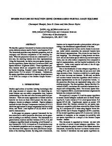
Table 3. Results on 2,4-D data The results showed that the classification error rate for the ordinary KNN was high for these complex data patterns. The ordinary KNN is sensitive to noisy data and does not rate the relative importance of individual features for discrimination. The performance of the GA/KNN hybrid approach was significantly better than the unmodified KNN. 3.3 Finding a Nearly Optimum Feature Set For the artificially generated dataset of Section IV.1, we found either the minimum or nearly minimum optimum feature set. However, for the real-world classification problems just discussed, it is not clear whether the GA/KNN solution is indeed the global optimal solution. We also noted in repeated runs of the GA/KNN on our biological datasets that the sets of weights found were not identical from run to run. This may reflect the fact that the minimum feature set required to distinguish the classes is not unique. We addressed these problems by further exploring the 2,4-D data using a number of variations on the original approach. The first of these was to perform 0/1 selection, then perform extraction on the reduced data set (called Selector-Distributor), in a two-step process. The first step, feature selection using wi ∈{0,1}, eliminates some features which are either noisy or contain insufficient or redundant information. The first step on the 2,4-D dataset reduced the number of features from 96 to 31. The error rate using selection alone was 0.83% In the second step, we used feature extraction in the range of [0,10] on the reduced set. For practical speedup of the GA, we set weight components less than 1 to zero. We ran the algorithm twice, using wi ∈[0, 10] range on a 31-feature set (based on the first selection result) and then on a 23-feature set (based on the second selection run). Both runs achieved an error rate of 0.24%, as shown in Figure 3. The best weight vector is shown in Table 4. We then examined the stepwise contribution of each element of the weight vector in their order of importance as indicated by the GA/KNN. Thus, we calculated and plotted the classification error rate of KNN using features x1*w 1; x1*w1 and x2*w2; x1*w1, x2*w2 and x3*w3; and so on respectively, in the order of w1>w2>w3>... . The result is shown in Figure 3.

.

feature # Weight feature # Weight

42

86

53

66

56

63

19

21

27

64

71

82

1.55 2.07 0.00 3.69 2.78 0.00 1.64 4.29 0.00 0.00 3.11 0.00 89

51

14

22

11

93

78

6

81

91

9

1.67 0.00 0.00 2.41 0.00 3.64 4.24 4.15 2.10 1.21 4.10

Table 4. Best weight vector for the 2,4-D data set From the above results we can draw this preliminary conclusion: feature selection and extraction as performed by the GA/KNN method can be used to find nearly minimum, nearly optimal feature sets for discrimination of at least some types of highdimensionality, noisy data. 3.4 Discovering New Features Using Nonlinear Transformation Having tested the approach on independent features, we examined the search capabilities of GA feature extraction using nonlinear transformations on correlated data. We investigated ways to use the correlations between fields in improving classifications. Of course, K nearest neighbor methods are sensitive to some inter-field correlations already, but not in the sharpest sense. If we know the form of some possibly significant inter-field correlations in advance, we can use that form of non-linear transformation to search for fields with those sorts of correlations. Not only would we do dimensionality reduction, but also creation of new meaningful features for effective classification. For example, we wondered whether, given a dataset in which a correlation between two otherwise non-discriminatory fields was important, the GA could discover the usefulness of that pairing in our scheme. An artificially generated dataset to test this hypothesis is shown in Table 5 .

19 42 91 81 86 89 22

71 66 6

56

93

9

78 21

Figure 3. 2,4-D feature importance analysis

The example data sets created using the template shown in Table 5 imply individual fields which are not by themselves significant for classification, but taken as pairs and multiplied together, completely separate the classes. The data consist of 15 independent uniform random values in the range [0.0 - 1.0] and two “hidden features” not appearing in the dataset; that is, the data were sieved to make the products of f1and f2, and of f3 and f4 significant, but no products actually appear among the data values. We believed it would be inefficient to create the fields for every combination of pairs of fields. This is because, for high-dimensionality data sets, the size of the chromosome would be very large (n genes for the features and n (n-1) for the pairs, for example). Instead, we coded some special fields, termed “index fields”, in the genome, representing pairs of field indices (instead of some weight) plus additional weight component fields to apply to these index-pair-generated terms. In this way, the GA can select the pair of fields to test for correlation under the predetermined transformation, and then weight, as it does all the other fields, the significance of that constructed feature. The evaluation function was modified such that values in the fields pointed to by the two indices would be passed through some pre-determined mathematical or logical operations (in this case, just simple multiplication). This essentially creates the product of these two fields as a new attribute of the individual to be classified. The GA can then search for a weight component for that product field. Only a tiny subset of all possible pairs of fields is being examined by the GA at any point in time, but whenever crossover or mutation alters an index pair, the GA essentially begins to search for a weight component for that new pair. For the runs to be discussed, only two weight values were possible for each index pair, represented by a single bit in the index part of the chromosome. The value of the weight component was set to either 10.0 or 0 depending on whether the weight component bit was on or off. We have conducted other experiments in which the GA searches through a large weight space, but this simpler approach seems to work very well, at least for these artificially generated test data. To allow a “selector of pairs” capability, if the GA chooses either index to be 0, then that index pair is not used in the evaluation function, thus allowing the GA to select for no index pair terms. The fitness function strongly discourages the use of the same index twice in a pair (e.g. 3,3) or the repetition of a pair in a string (e.g. 2, 5; 5, 2), by assigning a low fitness to any string with such a pair. The goal was to see if the GA, using the approach of searching simultaneously for index pairs and weight components on that pair, would discover the significant nonlinear transformation and work effectively. We modified the evaluation function as described, and allowed 3 index pairs at the end of each individual string of the population. We trained the algorithm on 10 examples from each of the 8 classes (80 total), then tested the trained algorithm on 1200 newly generated test examples. The results of running this modification are shown in Table 6. The GA indeed found the “hidden features” and therefore could perform classification. The pure KNN alone had an 88% error rate for the unknowns. The nonlinear transformation index algorithm did indeed find the appropriate indices in all of several runs and got the error rate down to 0.0% by finding the two index pairs (1,2) and (3,4), setting their weight components to 10, and dropping all other weight components to a low level shown on Table 6 and Table 7 respectively.

class

feature1~15

hidden feature 1

hidden feature 2

1

0.0~1.0

0.42 < (1) * (2) < 0.44

0.54 < (3) * (4) < 0.56

2

0.0~1.0

0.42 < (1) * (2) < 0.44

0.58 < (3) * (4) < 0.60

3

0.0~1.0

0.42 < (1) * (2) < 0.44

0.62 < (3) * (4) < 0.64

4

0.0~1.0

0.42 < (1) * (2) < 0.44

0.66 < (3) * (4) < 0.68

5

0.0~1.0

0.46 < (1) * (2) < 0.48

0.54 < (3) * (4) < 0.56

6

0.0~1.0

0.46 < (1) * (2) < 0.48

0.58 < (3) * (4) < 0.60

7

0.0~1.0

0.46 < (1) * (2) < 0.48

0.62 < (3) * (4) < 0.64

8

0.0~1.0

0.46 < (1) * (2) < 0.48

0.66 < (3) * (4) < 0.68

Table 5. Artificial test data template using hidden features Algorithm

population size

Trials

Error rate training set

Error rate 1200 test set

50

25,600

0.0%

0.58%

50

36,000

6.5%

22.67%

39.25%

86.75%

GA/KNN with index GA/KNN without index pure KNN

Table 6. Classification results of different approach field

field 1-15

weight component and index

0.0

field 16 field 17 field 18 10.0

10.0

0.0

index pair 1

index pair 2

index pair 3

1, 2

3, 4

5, 6

Table 7. Discovering a hidden feature using nonlinear transformation The goal was to see if the GA, using the approach of searching simultaneously for index pairs and weight components on that pair, would discover the significant nonlinear transformation and work effectively. We modified the evaluation function as described, and allowed 3 index pairs at the end of each individual string of the population. We trained the algorithm on 10 examples from each of the 8 classes (80 total), then tested the trained algorithm on 1200 newly generated test examples. The results of running this modification are shown in Table 6. The GA indeed found the “hidden fea-

tures” and therefore could perform classification. The pure KNN alone had an 88% error rate for the unknowns. The nonlinear transformation index algorithm did indeed find the appropriate indices in all of several runs and got the error rate down to 0.0% by finding the two index pairs (1,2) and (3,4), setting their weight components to 10, and dropping all other weight components to a low level shown on Table 6 and Table 7 respectively. This experiment tells us GA-based methods can be used to discover another transformation type, the definition of new derived attributes by applying mathematical or logical operators on the value of one or more fields in the data base. This makes it appear promising for many data mining applications.

4 Conclusions and Future Work In this paper we have shown that genetic algorithms can play an important role in the automated loop of feature extraction and of classification. The KNN classifier in the GA/KNN approach can be replaced by different other classifiers. We have also developed a GA/Rule for automatic feature extraction and classification using a production rule system. It has similar functionality and is more time efficient [10]. The basic model of feature extraction-feedback-classification technique also can be extended to apply to other data mining tasks such as association discovery, regression, or conceptual clustering if we can design appropriate criterion function. We believe genetic algorithms will be a useful tools for data mining in many situations. Acknowledgments This work was supported in part by Michigan State University’s Center for Microbial Ecology and the Beijing Natural Science Foundation of China. References [1] U. M. Fayyad, G. Piatetsky-Shapiro, P. Smyth, From Data Mining to Knowledge Discovery: An Overview, Advances in Knowledge Discovery and Data Mining, 1996, p1-34. [2] D. E. Goldberg. Genetic Algorithms in Search, Optimization and Machine Learning. New York: Addison Wesley, 1989. [3] W.F. Punch, E.D. Goodman, Min Pei, Lai Chia-shun, P.Hovland, and R. Enbody. Further Research on Feature Selection and Classification Using Genetic Algorithms. Proc. Fifth Inter. Conf. Genetic Algorithms and their Applications (ICGA), 1993, p.557. [4] Harry C. Andrew, Introduction to Mathematical Technique in Pattern Recognition. New York: John Wiley & Sons Inc. 1972. [5] W. Siedlecki and J. Sklansky, On Automatic Feature Selection Internat. Journal of Pattern Recognition and Artificial Intelligence. Vol 2, No.2 1988, 197-220. [6] A. K. Jain and B. Chandrasekaran, Dimensionality and Sample Size Considerations in Pattern Recognition Practice. Handbook of Statistics, Vol. 2 P. R. Krishnaiah and L. N. Kanal, eds. North-Holland, Amsterdam, 1982, 835-855 [7] A. Jain, Pattern Recognition. International Encyclopedia of Robotics Applications

and Automation, Wiley & Sons, 1988, 1052-1063. [8] P. A. Devijverand, J. Kittler, Pattern Recognition: A Statistical Approach, Prentice Hall, Lodon, 1982. [9] M. Pei, E.D. Goodman, W.F. Punch, Y. Ding, Genetic Algorithms for Classification and Feature Extraction. 1995 Annual Meeting, Classification Society of North America, June 1995. [10] M. Pei, E.D. Goodman, W.F. Punch, Pattern Discovery From Data Using Genetic Algorithms. First Pacific-Asia Conference on Knowledge Discovery & Data Mining, Feb. 1997.

Feature Extraction Using Genetic Algorithms M. Pei1, E. D. Goodman1, W. F. Punch2 1

Case Center for Computer-Aided Engineering and Manufacturing 2

Department of Computer Science Genetic Algorithms Research and Applications Group (GARAGe) Michigan State University, 2325 Engineering Building, East Lansing, MI 48824 e-mail: [email protected]

Abstract. This paper summarizes our research on feature selection and extraction from high-dimensionality data sets using genetic algorithms. We have developed a GA-based approach utilizing a feedback linkage between feature evaluation and classification. That is, we carry out feature selection or feature extraction simultaneously with classifier design, through “genetic learning and evolution.” This approach combines a GA with a classifier system. The classifier can be a standard K-Nearest-Neighbor decision rule, a production rule or another classifier. Here we use a K-Nearest-Neighbor classifier as an example to introduce this general method. We apply this approach on a series of artificial test data and on real-world biological data to show the utility of this approach.

1 Introduction The growing glut of data in the worlds of science, business and government create an urgent need for a new generation of automated and intelligent tools and techniques which can analyze, summarize, and extract “knowledge” from raw data [1]. Most knowledge discovery or data mining tools and techniques are based on statistics, machine learning, pattern recognition or artificial neural networks. The great challenge for data mining comes from huge databases of noisy, high-dimensionality data. Genetic algorithms (GAs) are good candidates for attacking this challenge since GAs are very useful for extracting patterns in multiclass, high-dimensionality problems where heuristic knowledge is sparse or incomplete [2] [3]. The data mining approach normally includes the three major steps in the knowledge discovery process: selection, cleaning, transformation and projection of data; mining the data to extract patterns; and evaluating and interpreting the results. The first step is data preprocessing, which is important before any learning or discovery algorithms of data mining are carried out. The key operation of data preprocessing is feature selection and extraction. Mining is only one step in the overall process. The quality of mined information depends not only on the effectiveness of the data mining technique used, but also on the quality and quantity of the data preprocessed. All of these steps are usually treated as independent on the path from data to knowledge, but any one step can result in changes in preceding or succeeding steps, often requiring starting from scratch with new choices and settings.

In this paper, we take classification as the main data mining task to show the general model of our approach. The data mining approach we have developed is based on a genetic algorithm which combines the preprocessing step of feature selection and extraction and the classification step into an automated loop. In a decision-theoretic or statistical approach to pattern recognition, the classification or description of data is based on the set of data features used. Therefore, feature selection and extraction are crucial in optimizing performance, and strongly affect classifier design. Defining appropriate features often requires interaction with experts in the application area. In practice, there is much noise and redundancy in most highdimensionality, complex patterns. Therefore, it is sometimes difficult even for experts to determine a minimum or optimum feature set. The “curse of dimensionality” becomes an annoying phenomenon in statistical pattern recognition, artificial neural network and other data-mining learning techniques. Researchers have discovered that many learning procedures lack the property of “scalability” -- i.e., these procedures either fail or produce unsatisfactory results when applied to problems of larger size[6] [7] [8]. To address this scalability problem, we present an approach for automatic feature selection and extraction using genetic algorithms (GA’s). The basic operation of this approach utilizes a feedback linkage between feature evaluation and classification. That is, we carry out feature transformation and classifier design simultaneously, through “genetic learning and evolution.” The objective of this approach is to find a reduced subset among the original N features such that useful class discriminatory information is included and redundant class information and/or noise is excluded. We take the following general approach. The data’s original feature space is transformed into a new feature space with fewer features that (potentially) offer better separation of the pattern classes, which, in turn, improves the performance of the decision-making classifier. The criterion for optimality of the feature subset selected is usually the probability of misclassification. Since the number of different subsets of N available features can be very large, exhaustive search is computationally infeasible and other methods must be examined. In the field of pattern recognition, a number of heuristic techniques have been used, but it is not clear under what circumstances any one heuristic should be applied, as each has its good and bad points. In order to apply a GA to classification/discrimination tasks and work out feature transformations, we combine the GA with a K Nearest Neighbor decision rule, calling the result the GA/KNN hybrid approach. Here the GA defines a population of weight vectors w*, where the dimension of each w* is the dimension of the data pattern x for each example. Each w* from the GA is multiplied with every sample’s data pattern vector x, yielding a new feature vector y for the given data. The KNN algorithm then classifies the entire y-transformed data set. The results of the classification for a known “training” sample set are fed back as part of the fitness function, to guide the genetic learning/search for the best transformation. The GA result is the “best” vector w* under the (potentially conflicting) constraints of the evaluation function. For example, the “best” w* might be both parsimonious (have the fewest features) and give the fewest misclassifications. Thus, the GA searches for an optimal transformation from the original pattern space to feature space for improving the performance of the KNN clas-

sifier[3]. In the following sections, we describe the basic concepts of our approach; present the GA/KNN approach in more detail; show the results of several experiments; then finally propose some brief conclusions and offer areas of future study.

2 GA/KNN Hybrid Approach 2.1 Basic Concept of the Approach In the design of automatic pattern classifiers, ideally the problem of feature selection and extraction on the one hand and the classifier design on the other should not be considered independently. Yet, for practical considerations, most researchers make the simplifying assumption that the feature selection/extraction stage and the classification stage are independent. However the ultimate goal is correct classification with a corresponding feature pattern extracted and the intermediate step of feature extraction and dimensionality reduction is, in a sense, subservient to that goal and is not an end in itself. It would be better to couple feature selection/extraction with effective classification techniques[4]. This implies some sort of classification decision feedback mechanism to modify or adapt the feature extractor. Our research follows this direction. The approach which adopt the above idea is a supervised induction, i.e. “genetic learning and evolution,” as shown in Figure 1. N=Finite dimensional

K = number of classes Feature Extractor

Pattern Space

Classifier Feature Space Genetic learning and Evolution

Classification Space

Feedback

Figure 1. Feature Extractor and Classifier with Feedback Learning System In the GA/KNN hybrid approach, as mentioned above, a genetic algorithm using a K Nearest Neighbor decision rule searches for a “best” diagonal matrix [W] or weight vector w* -- i.e., a “best” transformation from pattern space to feature space for improving the performance of the KNN classifier [3] -- under potentially conflicting constraints of the evaluation function. The whole structure of the GA/KNN hybrid approach is shown in Figure 2. 2.2 Different Transformations Using a GA Based on the above discussion of a GA approach to feature extraction, we formally

describe the problem by defining the mapping function M() and criterion function J().

. Initialize Population (random set of weights w*) New Population

Training x data set

y = M(x) = W x Evaluate by KNN Rule

Yes

Satisfy?

No GA

Evolution Selection Crossover

Best set of weights w*

Mutation

Figure 2. The structure of GA/KNN approach We define w*, the weight vector, to be a N = |x| vector (or NxN diagonal matrix [W]) generated by the GA, to multiply each pattern vector x, yielding the new feature vector y. That is, (1) linear transformation y = M(x) = Wx where

...˙ 0 0 w 2 ... 0 . . . . . , or w* = [w1,w2, …, wΝ], . . . . .

w1 0 W =

x = [x1, x2, ⋅ ⋅ ⋅ , xN]

0 0 0 0 wN

• wi ∈{0,1}, 1≤ i ≤Ν. When we use only binary values for w*, we interpret it as follows: if the ith weight

component is one, then the ith feature is preserved in feature space; otherwise, the feature is discarded from the feature set. Thus we perform feature selection to define an optimal subset and (potentially) reduce the dimensionality of the original data pattern[5]. • wi ∈[a, b], such that wi ∈[0.0, 10.0] 1≤ i ≤Ν. We can instead do feature extraction by allowing the values of the weight components to range over some values [a, b], such as 0.0 to 10.0 (presuming that the features are first “normalized” to some standard range). That amounts to searching for a relative weighting of features that gives optimal performance on classification of the known samples. Thus we are selecting for features in a linearly transformed space. Those weight components that move towards 0 indicate that their corresponding features are not important for the discrimination task. Essentially, those features “drop out” of the feature space and are not considered. Any feature that moves towards the maximum weight indicates that the classification process is sensitive to changes in that feature. That feature’s dimension is elongated, which probably reflects that an increased separation between the classes gave better resolution. The resulting weights indicate the usefulness of a particular feature, sometimes called its discriminatory power.[4][8] Usually, only feature selection can reduce the overall cost of measurement acquisition, since feature extraction utilizes all information in the pattern representation vector x to yield feature vector y of lower dimension. But in the case above, the simple diagonal transformation certainly can reduce the cost of measurement. (2) nonlinear transformation, as, for example: y = M(x) = Wx* where

x* = [x1, x2, ⋅ ⋅ ⋅ , xN, (xi•xj)1, (xn•xm)2, ⋅ ⋅ ⋅ , (xr•xs)k], for example, ˙ 0 ... 0 w 2 ... 0 . . . . . 0 . . . . 0. 0

w1 0 W =

, or

w* = [w1,w2, …, wΝ, wN+1, …, wN+k ],

0 0 0 0 wN + k

The previous linear transformation can mainly be used on data patterns with classes which are linearly separable based on scaling or other linear operations. However, linear transformations are not necessarily sufficient for effective feature selection and extraction, so an extended form of the above linear transformation is used here. We have investigated the use of nonlinear transformations to address the feature extraction and subsequent classification of data patterns, where those data patterns have correlations between different feature fields. This approach is based on an a priori knowledge of possible forms of the relationship of the features and the use of a GA to discover which of those forms best captures the relationship.

The various combinations (xi•xj)1, (xn•xm)2, ⋅ ⋅ ⋅ , (xr•xs)k in x* form a set of new features which can be constructed and discovered by performing various mathematical or logical operations. Choice of appropriate combinations is obviously problem dependent. In our experiments, we tested an example data pattern which consists of 15 features, any feature of which by itself is not discriminatory but which does contain two combinations of features which are discriminatory. The search problem is NP hard[5]. Originally, for even moderate numbers of features (say between 15 and 30) the problem must be solved with the aid of suboptimal heuristic methods. These methods, by definition, do not ensure that the result is optimal. Genetic algorithms are good candidates for this task, since GAs search from a population, not a single point, and discover new solutions by speculating on many combinations of the best partial solutions (called building blocks) contained within the current population. GAs are most useful in multiclass, high-dimensionality problems in which guarantees on the performance of heuristics are sparse or inadequate. GA’s are considered to be global search methods.There are several problems in running a GA/KNN approach for feature extraction which must be addressed, such as: chromosome encoding representation, normalization of training data, and fitness function design. We do not discuss them in detail here; interested reader can refer to [9]. There are several problems in running a GA/KNN approach for feature extraction which must be addressed, such as: chromosome encoding representation, normalization of training data, and fitness function design. We do not discuss them in detail here; interested reader can refer to [9].

3 Test Results of GA/KNN Hybrid Approach 3.1 Artificially Generated Datasets Our first work used several artificially generated data sets, of which Table 1 is typical. The table represents a template from which we generated as many examples as needed. The expression {0.0 - 1.0} represents uniform random values generated in the range of 0.0 to 1.0. The expression 0.5+5∗[f3]2 represents a generation expression where [f3] means that the present value of the f3 field is used in the calculation. Thus field f1 and f7 - f15 represent uniform random noise generated in the range {0.0 - 1.0}, while f2 f6 are fields that can be used to distinguish the eight classes A - H, where fields f4 and f5 make use of values generated in f3. Note that using uniform random values up to contiguous field boundaries (in contrast to normally distributed values with a specified mean and variance) yields a dataset much harder for a KNN to classify than (for example) for an algorithm based on discrete thresholds. The encoding string (chromosome) length for the GA for this data set was (15∗1) =15 bits for feature selection and (15∗8) = 120 bits for feature extraction. The population size used was 50. The parameters used to run the GA were two-point crossover with probability: 0.60 ~ 0.80, mutation rate: 0.001 per bit. The GA was “trained” on a set of 30 examples of each of the 8 pattern classes for a total of 240 examples. The GA was run on the 240 exemplars until the population

converged. This “best” w* was then evaluated on a set of 1200 new examples generated by the same template. Two typical such w*, in the ranges of {0, 1} and [0.0 - 10.0] respectively, are shown in Table 2. Note that the irrelevant features were removed (set to 0) by both feature selection and feature extraction. The performance of the discovered w* on classification of the unknown set is also shown in Table 2. The percentages listed are averages of 5 runs and compare a number of variations on the basic approach. Note that in classifying the training data, the KNN evaluation function was modified so as to not use the point being tested as its own “neighbor”. This “leave-oneout” strategy was used make the training data resemble the test data more closely, since a test datum will not have itself as a near neighbor during KNN evaluation. Note the distinct improvement of the transformed space over the standard and normalized spaces using a KNN alone. Further note that the results of selection (wi ∈{0,1} weighting) and extraction (wi ∈[0, 10] weighting) are quite similar. The results of the 0-10 weighting would have been better, but appeared to settle at a local minimum. This was likely due to the small signal/noise ratio of the artificially generated, uniformly random dataset. This is supported by the experiment in which we ran the 0/1 weighting as a feature selection filter, followed by the 0-10 weightings, in which we obtained a much better result (3% error) . class field 1 field 2 field 3 field 4 field 5 field 6 field7~15 A B C

0.0~1.0 0.0~1.0 0.0~1.0

0.0~1.0

0.0~0.1

0.0~1.0

0.0~0.1

0.0~1.0

0.1~0.2

0.2+[f3] 0.5∗[f3]2 0.5+5∗[f3]2

0.0~1.0

0.2+[f3]

0.5∗[f3]2

1.0-25∗[f3]2

0.0~1.0

0.3--[f3]

0.5∗[f3]2

0.5+5∗[f3]2

0.0~1.0

0.5∗[f3]2

1.0-25∗[f3]2

0.0~1.0

D

0.0~1.0

0.0~1.0

0.1~0.2

0.3--[f3]

E

0.0~1.0

0.1~0.2

0.0~0.1

0.2+[f3] 0.5∗[f3]2 0.5+5∗[f3]2

0.0~1.0

F

0.0~1.0

0.1~0.2

0.0~0.1

0.2+[f3] 0.5∗[f3]2 1.0-25∗[f3]2

0.0~1.0

G

0.0~1.0

0.1~0.2

0.1~0.2

0.3--[f3] 0.5∗[f3]2 0.5+5∗[f3]2

0.0~1.0

H

0.0~1.0

0.1~0.2

0.1~0.2

0.3--[f3]

0.5∗[f3]2

1.0-25∗[f3]2

0.0~1.0

Table 1. A template for artificially generated datasets Errors # of unknown normalized patterns KNN 1200 35.93% Type of w* wi ∈{0,1} wi ∈[0, 10]

f1 0 0.000

Errors 0/1 weighted KNN 6.4%

f2 1 5.154

f3 1 4.656

Errors 0~10 weighted KNN 4.13% f4 1 7.622

f5 0 0.000

Errors 0~10 weighted KNN after selection 3.0% f6 1 4.248

Table 2. Results on artificially generated datasets

f7-f15 0 0.000

We have compared our approach with Whitney’s method (estimation of k-NN classification error by the method of leave-one-out and sequential forward selection) on this artificially generated data set. The results of that method appear quite poor. The classification error rate was 95% for the 8-class data set. This suboptimal method is essentially useless in this case. 3.2 A Real-World Problem -- Biological Pattern Classification. Having established the usefulness of GA feature selection and extraction on various test data, we explored classification of several real-world datasets exemplifying highdimensionality biological data. Researchers in the Center for Microbial Ecology (CME) of Michigan State University have sampled various agricultural environments for study. Their first experiments used the Biolog test as the discriminator. Biolog consists of a plate of 96 wells, with a different substrate in each well. These substrates (various sugars, amino acids and other nutrients) are assimilated by some microbes and not by others. If the microbial sample processes the substrate in the well, that well changes color, which can be recorded photometrically. Thus large numbers of samples can be processed and characterized based on the substrates they can assimilate. Each microbial sample described was tested on the 96 features provided by Biolog (for some experiments, extra taxonomic data were also used); the value of each feature is either 0 or 1. Using the Biolog test suite to generate data, the test set called 2,4-D data set is used in showing the effectiveness of our approach. 2,4-D Data Set Soil samples were collected from a site that is contaminated with 2,4-D (dichlorophenoxyacetic acid), a pesticide. There are 3 classes, based on three genetically similar microbial isolates which show the ability to degrade 2,4-D. There were are a total of 232 samples. The questions to be asked using this experiment were of two types: 1. Classification and prediction -- whether these samples from different environments could be distinguished. 2. Identification. Which of the available features are most important for the discrimination and which are acting primarily as “noise” - that is, non-contributing features. We applied our GA/KNN hybrid method on the type of biological data set described above. Each data element was a 96-bit vector, in which a positive result was a represented by a 1 and a negative result, a 0. In other words, the data elements form dichotomous measurement spaces, or binary pattern spaces. When doing feature selection, the chromosome was, correspondingly, a 96-bit binary vector, indicating feature used or not used. When we used a GA to search for a best transformation weight vector, the length of string (chromosome) was a considerably longer (8*96) = 768. Compared with the large number of features, the available training data were limited, since there were 241 samples in the data set. All samples were used in leave-one-out training, then 10 randomly selected subsets of the training data were tested and results aver-

aged. The classification results of this experiments are listed in Table 3. number of patterns

Errors, with original Knn

Errors, with 0/1 weighted Knn

Errors, with 0-10 weighted Knn

test 10%

8.30%

3.20%

2.00%

training 232

6.64%

1.66%

0.83%

Table 3. Results on 2,4-D data The results showed that the classification error rate for the ordinary KNN was high for these complex data patterns. The ordinary KNN is sensitive to noisy data and does not rate the relative importance of individual features for discrimination. The performance of the GA/KNN hybrid approach was significantly better than the unmodified KNN. 3.3 Finding a Nearly Optimum Feature Set For the artificially generated dataset of Section IV.1, we found either the minimum or nearly minimum optimum feature set. However, for the real-world classification problems just discussed, it is not clear whether the GA/KNN solution is indeed the global optimal solution. We also noted in repeated runs of the GA/KNN on our biological datasets that the sets of weights found were not identical from run to run. This may reflect the fact that the minimum feature set required to distinguish the classes is not unique. We addressed these problems by further exploring the 2,4-D data using a number of variations on the original approach. The first of these was to perform 0/1 selection, then perform extraction on the reduced data set (called Selector-Distributor), in a two-step process. The first step, feature selection using wi ∈{0,1}, eliminates some features which are either noisy or contain insufficient or redundant information. The first step on the 2,4-D dataset reduced the number of features from 96 to 31. The error rate using selection alone was 0.83% In the second step, we used feature extraction in the range of [0,10] on the reduced set. For practical speedup of the GA, we set weight components less than 1 to zero. We ran the algorithm twice, using wi ∈[0, 10] range on a 31-feature set (based on the first selection result) and then on a 23-feature set (based on the second selection run). Both runs achieved an error rate of 0.24%, as shown in Figure 3. The best weight vector is shown in Table 4. We then examined the stepwise contribution of each element of the weight vector in their order of importance as indicated by the GA/KNN. Thus, we calculated and plotted the classification error rate of KNN using features x1*w 1; x1*w1 and x2*w2; x1*w1, x2*w2 and x3*w3; and so on respectively, in the order of w1>w2>w3>... . The result is shown in Figure 3.

.

feature # Weight feature # Weight

42

86

53

66

56

63

19

21

27

64

71

82

1.55 2.07 0.00 3.69 2.78 0.00 1.64 4.29 0.00 0.00 3.11 0.00 89

51

14

22

11

93

78

6

81

91

9

1.67 0.00 0.00 2.41 0.00 3.64 4.24 4.15 2.10 1.21 4.10

Table 4. Best weight vector for the 2,4-D data set From the above results we can draw this preliminary conclusion: feature selection and extraction as performed by the GA/KNN method can be used to find nearly minimum, nearly optimal feature sets for discrimination of at least some types of highdimensionality, noisy data. 3.4 Discovering New Features Using Nonlinear Transformation Having tested the approach on independent features, we examined the search capabilities of GA feature extraction using nonlinear transformations on correlated data. We investigated ways to use the correlations between fields in improving classifications. Of course, K nearest neighbor methods are sensitive to some inter-field correlations already, but not in the sharpest sense. If we know the form of some possibly significant inter-field correlations in advance, we can use that form of non-linear transformation to search for fields with those sorts of correlations. Not only would we do dimensionality reduction, but also creation of new meaningful features for effective classification. For example, we wondered whether, given a dataset in which a correlation between two otherwise non-discriminatory fields was important, the GA could discover the usefulness of that pairing in our scheme. An artificially generated dataset to test this hypothesis is shown in Table 5 .

19 42 91 81 86 89 22

71 66 6

56

93

9

78 21

Figure 3. 2,4-D feature importance analysis

The example data sets created using the template shown in Table 5 imply individual fields which are not by themselves significant for classification, but taken as pairs and multiplied together, completely separate the classes. The data consist of 15 independent uniform random values in the range [0.0 - 1.0] and two “hidden features” not appearing in the dataset; that is, the data were sieved to make the products of f1and f2, and of f3 and f4 significant, but no products actually appear among the data values. We believed it would be inefficient to create the fields for every combination of pairs of fields. This is because, for high-dimensionality data sets, the size of the chromosome would be very large (n genes for the features and n (n-1) for the pairs, for example). Instead, we coded some special fields, termed “index fields”, in the genome, representing pairs of field indices (instead of some weight) plus additional weight component fields to apply to these index-pair-generated terms. In this way, the GA can select the pair of fields to test for correlation under the predetermined transformation, and then weight, as it does all the other fields, the significance of that constructed feature. The evaluation function was modified such that values in the fields pointed to by the two indices would be passed through some pre-determined mathematical or logical operations (in this case, just simple multiplication). This essentially creates the product of these two fields as a new attribute of the individual to be classified. The GA can then search for a weight component for that product field. Only a tiny subset of all possible pairs of fields is being examined by the GA at any point in time, but whenever crossover or mutation alters an index pair, the GA essentially begins to search for a weight component for that new pair. For the runs to be discussed, only two weight values were possible for each index pair, represented by a single bit in the index part of the chromosome. The value of the weight component was set to either 10.0 or 0 depending on whether the weight component bit was on or off. We have conducted other experiments in which the GA searches through a large weight space, but this simpler approach seems to work very well, at least for these artificially generated test data. To allow a “selector of pairs” capability, if the GA chooses either index to be 0, then that index pair is not used in the evaluation function, thus allowing the GA to select for no index pair terms. The fitness function strongly discourages the use of the same index twice in a pair (e.g. 3,3) or the repetition of a pair in a string (e.g. 2, 5; 5, 2), by assigning a low fitness to any string with such a pair. The goal was to see if the GA, using the approach of searching simultaneously for index pairs and weight components on that pair, would discover the significant nonlinear transformation and work effectively. We modified the evaluation function as described, and allowed 3 index pairs at the end of each individual string of the population. We trained the algorithm on 10 examples from each of the 8 classes (80 total), then tested the trained algorithm on 1200 newly generated test examples. The results of running this modification are shown in Table 6. The GA indeed found the “hidden features” and therefore could perform classification. The pure KNN alone had an 88% error rate for the unknowns. The nonlinear transformation index algorithm did indeed find the appropriate indices in all of several runs and got the error rate down to 0.0% by finding the two index pairs (1,2) and (3,4), setting their weight components to 10, and dropping all other weight components to a low level shown on Table 6 and Table 7 respectively.

class

feature1~15

hidden feature 1

hidden feature 2

1

0.0~1.0

0.42 < (1) * (2) < 0.44

0.54 < (3) * (4) < 0.56

2

0.0~1.0

0.42 < (1) * (2) < 0.44

0.58 < (3) * (4) < 0.60

3

0.0~1.0

0.42 < (1) * (2) < 0.44

0.62 < (3) * (4) < 0.64

4

0.0~1.0

0.42 < (1) * (2) < 0.44

0.66 < (3) * (4) < 0.68

5

0.0~1.0

0.46 < (1) * (2) < 0.48

0.54 < (3) * (4) < 0.56

6

0.0~1.0

0.46 < (1) * (2) < 0.48

0.58 < (3) * (4) < 0.60

7

0.0~1.0

0.46 < (1) * (2) < 0.48

0.62 < (3) * (4) < 0.64

8

0.0~1.0

0.46 < (1) * (2) < 0.48

0.66 < (3) * (4) < 0.68

Table 5. Artificial test data template using hidden features Algorithm

population size

Trials

Error rate training set

Error rate 1200 test set

50

25,600

0.0%

0.58%

50

36,000

6.5%

22.67%

39.25%

86.75%

GA/KNN with index GA/KNN without index pure KNN

Table 6. Classification results of different approach field

field 1-15

weight component and index

0.0

field 16 field 17 field 18 10.0

10.0

0.0

index pair 1

index pair 2

index pair 3

1, 2

3, 4

5, 6

Table 7. Discovering a hidden feature using nonlinear transformation The goal was to see if the GA, using the approach of searching simultaneously for index pairs and weight components on that pair, would discover the significant nonlinear transformation and work effectively. We modified the evaluation function as described, and allowed 3 index pairs at the end of each individual string of the population. We trained the algorithm on 10 examples from each of the 8 classes (80 total), then tested the trained algorithm on 1200 newly generated test examples. The results of running this modification are shown in Table 6. The GA indeed found the “hidden fea-

tures” and therefore could perform classification. The pure KNN alone had an 88% error rate for the unknowns. The nonlinear transformation index algorithm did indeed find the appropriate indices in all of several runs and got the error rate down to 0.0% by finding the two index pairs (1,2) and (3,4), setting their weight components to 10, and dropping all other weight components to a low level shown on Table 6 and Table 7 respectively. This experiment tells us GA-based methods can be used to discover another transformation type, the definition of new derived attributes by applying mathematical or logical operators on the value of one or more fields in the data base. This makes it appear promising for many data mining applications.

4 Conclusions and Future Work In this paper we have shown that genetic algorithms can play an important role in the automated loop of feature extraction and of classification. The KNN classifier in the GA/KNN approach can be replaced by different other classifiers. We have also developed a GA/Rule for automatic feature extraction and classification using a production rule system. It has similar functionality and is more time efficient [10]. The basic model of feature extraction-feedback-classification technique also can be extended to apply to other data mining tasks such as association discovery, regression, or conceptual clustering if we can design appropriate criterion function. We believe genetic algorithms will be a useful tools for data mining in many situations. Acknowledgments This work was supported in part by Michigan State University’s Center for Microbial Ecology and the Beijing Natural Science Foundation of China. References [1] U. M. Fayyad, G. Piatetsky-Shapiro, P. Smyth, From Data Mining to Knowledge Discovery: An Overview, Advances in Knowledge Discovery and Data Mining, 1996, p1-34. [2] D. E. Goldberg. Genetic Algorithms in Search, Optimization and Machine Learning. New York: Addison Wesley, 1989. [3] W.F. Punch, E.D. Goodman, Min Pei, Lai Chia-shun, P.Hovland, and R. Enbody. Further Research on Feature Selection and Classification Using Genetic Algorithms. Proc. Fifth Inter. Conf. Genetic Algorithms and their Applications (ICGA), 1993, p.557. [4] Harry C. Andrew, Introduction to Mathematical Technique in Pattern Recognition. New York: John Wiley & Sons Inc. 1972. [5] W. Siedlecki and J. Sklansky, On Automatic Feature Selection Internat. Journal of Pattern Recognition and Artificial Intelligence. Vol 2, No.2 1988, 197-220. [6] A. K. Jain and B. Chandrasekaran, Dimensionality and Sample Size Considerations in Pattern Recognition Practice. Handbook of Statistics, Vol. 2 P. R. Krishnaiah and L. N. Kanal, eds. North-Holland, Amsterdam, 1982, 835-855 [7] A. Jain, Pattern Recognition. International Encyclopedia of Robotics Applications

and Automation, Wiley & Sons, 1988, 1052-1063. [8] P. A. Devijverand, J. Kittler, Pattern Recognition: A Statistical Approach, Prentice Hall, Lodon, 1982. [9] M. Pei, E.D. Goodman, W.F. Punch, Y. Ding, Genetic Algorithms for Classification and Feature Extraction. 1995 Annual Meeting, Classification Society of North America, June 1995. [10] M. Pei, E.D. Goodman, W.F. Punch, Pattern Discovery From Data Using Genetic Algorithms. First Pacific-Asia Conference on Knowledge Discovery & Data Mining, Feb. 1997.