An Optimal Sensing Framework Based on Spatial RSS ... - CiteSeerX

An Optimal Sensing Framework Based on Spatial RSS-profile in Cognitive Radio Networks Alexander W. Min and Kang G. Shin Real-Time Computing Laboratory, Dept. of EECS The University of Michigan, Ann Arbor, MI 48109-2121 {alexmin,kgshin}@eecs.umich.edu Abstract—In cognitive radio networks (CRNs), regulatory bodies, such as the FCC, enforce an extremely demanding detectability requirement to protect primary users’ communications, which can hardly be achieved with one-time sensing using only a single sensor. Most of the previous work focused on either cooperative sensing or sensing scheduling as a viable means to improve the detection performance without studying their interactions. In this paper, we propose an optimal spectrum sensing framework in CRNs that jointly exploits sensors’ cooperation and sensing scheduling to meet the desired detection performance with minimum sensing overhead. Specifically, we propose an optimal sensing framework for the IEEE 802.22 wireless regional area networks (WRANs) that directs the base station (BS) to manage spectrum sensing by (i) constructing each primary signal’s spatial profile of received signal strengths (RSSs) as a detection criterion, (ii) selecting an optimal set of sensors for cooperative sensing, and (iii) finding an optimal time to stop sensing. This framework will ensure the desired sensing performance of 802.22 with minimum sensing overhead. Our evaluation results show that the proposed sensing algorithms reduce the sensing overhead significantly and lower the feasible operation region of energy detector by 13 dB for practical scenarios.

I. I NTRODUCTION In cognitive radio networks (CRNs), spectrum sensing is a key component that enables opportunistic spectrum access while preventing any unacceptable interference to primary communications. To protect primary signals from interference, sensing must meet strict requirements set by the FCC. For example, in IEEE 802.22 WRANs [1], any primary signal above the incumbent detection threshold (IDT), e.g., −116 dBm for the DTV signal, must be detected with both false-alarm and miss-detection probabilities less than 0.1 [2]. Unfortunately, this stringent performance requirement cannot be met with one-time sensing with a single sensor regardless of the underlying sensing technique, e.g., energy/feature detection [3]–[5]. Thus, in order to compensate for the performance deficiency of existing sensing techniques, the number of sensed samples can be increased by (i) having multiple sensors cooperate (in spatial domain) and/or (ii) scheduling sensing events (in temporal domain). Cooperative sensing has been studied extensively as a viable means to improve the sensing performance [6]–[12], where multiple sensors monitor the spectrum individually during the quiet period and then transmit their sensing results to a central node (e.g., the base station) for the final decision. To derive an optimal decision, different sensitivities of sensors should be considered in data (or decision) fusion [6], [9]. These heterogeneous sensitivities often stem from the geographical locations of sensors and the existence of channel fading,

e.g., multi-path or shadowing, thus making sensors experience different received signal strengths (RSSs) of a primary signal [7]–[11]. In this paper, we refer to these heterogeneous RSSs among sensors as spatial RSS diversity. The main goal of cooperative sensing is to improve detection performance by maximally exploiting the spatial RSS diversity among sensors. However, the cooperation gain has been reported to degrade as the shadowing correlation among sensors increases [7], [9], [10]. To minimize the detrimental effects of shadow correlation on cooperative sensing, several sensor-selection algorithms have been introduced. For example, Sel´en et al. [13] proposed heuristic algorithms for selecting an uncorrelated set of sensors given different degrees of information about sensor locations. Similarly, Kim and Shin [14] suggested to select sensors based on their geographical separation so as to make the sensors uncorrelated from each other. However, these sensor selection methods incur significant overheads in measuring the actual shadowing correlation among sensors or may require the deployment of additional sensors to achieve uncorrelated sensing results. Scheduling sensing also aims to improve the detection performance by sensing a channel multiple times, and thus, exploiting temporal variations in RSSs at each sensor. For example, in 802.22, a base station can schedule the quiet period for energy detection multiple times within the channel detection time (CDT) and take into account those sensing results to enhance the overall incumbent detection performance [15]. However, during the quiet period, all the secondary users must remain silent, thus wasting precious resources, such as energy and time, and degrading the quality-of-service (QoS) of secondary communications. The quiet period, therefore, must be optimally scheduled so as to minimize the sensing-time while guaranteeing the required sensing performance. Despite its importance, this optimal sensing scheduling only recently started to receive attention. For example, Lee and Akyildiz [16] proposed an optimization framework for spectrum selection and scheduling subject to interference constraints. Kim and Shin [14] developed a lookup-tablebased offline sensing scheduling algorithm for in-band sensing in 802.22. Huang et al. [17] studied an optimal sensingtransmission policy to maximize a secondary user’s utility. In the IEEE 802.22 standard draft, a two-stage sensing mechanism has been proposed to provide flexible scheduling of quiet periods [18]. However, none of these scheduling algorithms is optimal in the sense of minimizing the number of sensing periods. More importantly, the interactions between cooperative sensing and sensing scheduling have not been studied.

In this paper, we propose an efficient spectrum-sensing framework for the IEEE 802.22 that jointly exploits spatial and temporal RSS variations to minimize the sensing overhead subject to the sensing performance requirement of 802.22. In particular, we address the following important issues in spectrum sensing: (i) which sensors to use for cooperative sensing, (ii) how to incorporate their heterogeneous sensitivities in data fusion, and (iii) how to adaptively schedule in-band sensing to minimize the sensing overhead. A. Contributions This paper makes the following main contributions. • Introduction of a new concept of spatial RSS-signaturebased cooperative sensing that exploits the spatial variations in RSSs among cooperating sensors by learning the RSS distributions at sensor locations. This is a feasible and useful approach in CRNs where sensor locations are stationary, thus making their RSS distributions unique and (pseudo) time-invariant. • Development of a simple and near-optimal linear datafusion rule for detection of a primary signal based on a one-time sensing via a linear discriminant analysis (LDA). This is based on the observation that, when energy detection is employed in a low SNR environment such as IEEE 802.22 WRANs, spatial RSS distributions can be approximated as multi-dimensional Gaussian with a common covariance matrix. The theoretical performance of LDA-based decision rule under shadow fading is also presented. • Proposal of an optimization framework for minimizing the sensing overhead of cooperative sensing, which consists of: (i) an algorithm for selecting an optimal set of sensors for cooperative sensing (Section IV-B), and (ii) an online sensing-period scheduling algorithm that finds an optimal stopping time via a sequential probability ratio test (SPRT) based on the sensing results (Section IV-A). • In-depth simulation to demonstrate the benefits of the proposed spectrum-sensing algorithms. Our simulation results show that the proposed RSS-profile-based detection schemes for both one-time (i.e., LDA-based) and sequential (i.e., SPRT-based) sensing significantly improve detection performance over the conventional decision fusion rules, such as the OR-rule.1 The results also show that our algorithms for sensor selection reduces the average sensing overhead significantly.

II. P RELIMINARIES In this section, we first briefly introduce the IEEE 802.22 wireless regional area network (WRAN), including its performance requirements for spectrum sensing. We then review the spectrum sensing and energy detection in 802.22, and outline the proposed RSS-profile-based cooperative sensing. A. IEEE 802.22 WRANs We consider the IEEE 802.22 WRAN [1], an infrastructurebased wireless air interface, in which each cell is composed of a base station (BS) and the associated end-users called consumer premise equipment (CPE). Secondary devices in IEEE 802.22 seek spectrum opportunities (white spaces) on VHF/UHF bands. Among different types of incumbent signals (i.e., NTSC, DTV, and wireless microphones), we focus on detecting DTV signals, although our approach can be extended to include detection of other types of primary signals, such as analog TV and wireless microphone signals. To protect primary users (i.e., TV receivers), CPEs should be located outside the keep-out radius of 150.3 km from the TV transmitter [20]. In general, CPEs (i.e., houses) are static2 and form various clusters of different sizes. At the edge of the keep-out radius, the DTV signal power is attenuated to −96.5 dBm, which is below the average noise power, i.e., −95.2 dBm [20]. The IEEE 802.22 standard draft has numerical performance requirements on spectrum sensing in terms of: (i) minimum signal power, (ii) detection delay, and (iii) sensing accuracy [21]. First, sensing must be able to detect the incumbent signals with signal strength above the incumbent detection threshold (IDT), e.g., −116 dBm for the DTV signal. Second, sensing must be fast enough to detect the primary signal within the channel detection time (CDT) (for in-band sensing) of 2 seconds after its appearance. Third, sensing must be accurate to guarantee the probabilities of false alarm and miss detection below certain thresholds, i.e., PF A ≤ 0.1 and PMD ≤ 0.1, for any primary signal stronger than the IDT.

B. Organization The remainder of this paper is organized as follows. Section II briefly reviews the IEEE 802.22 WRAN and the energydetection technique, followed by our approach to exploiting the spatio-temporal variations in RSSs for spectrum sensing. Section III presents our RSS-signature-based detection scheme for one-time sensing and its theoretical performance. Section IV introduces our cooperative sensing algorithms designed to (i) select an optimal set of sensors and (ii) find an optimal time to stop sensing. Section V evaluates the performance of the proposed algorithms, and Section VI concludes the paper.

B. Spectrum Sensing in IEEE 802.22 The IEEE 802.22 standard draft employs a distributed spectrum sensing (DSS) where CPEs are required to report their local sensing results to the BS [12]. It also provides a two-stage sensing (TSS) mechanism to schedule quiet periods (QPs) for in-band sensing [15]. According to the TSS, the BS can schedule QPs multiple times for fast-sensing (i.e., energy detection) within each CDT [2]. Then, based on the fast-sensing results, the BS determines the need to schedule a longer QP for fine-sensing (i.e., feature detection) at the end of a CDT in order to obtain more accurate sensing results. However, the current 802.22 draft does not specify any algorithm for efficient scheduling of QPs, or how to select sensors for cooperation. Therefore, we have opted to develop an online QP scheduling algorithm for fast-sensing that finds an optimal stopping time for QPs to minimize the sensing overhead while guaranteeing the detection requirements of 802.22. We also propose an algorithm to find an optimal set of sensors for cooperative sensing by exploiting sensor heterogeneity (in detectability) due to different sensor locations.

1 The OR-rule is the most common decision-fusion rule in the absence of prior knowledge of RSS distributions [3], [7], [12], [14], [19].

2 In 802.22, secondary devices are required to be stationary in order to prevent potential interference to primary communications due to mobility.

where yi (n) is the signal received by a secondary user, si (n) is the primary signal, and wi (n) is an i.i.d. additive white Gaussian noise (AWGN), at sensor i in the nth time slot within the sensing duration. Thus, the test statistic of the energy detector is an estimate of average RSS [3]: Ti =

M B X yi (n) ∗ yi (n), M n=1

(1)

where B is the channel bandwidth (e.g., 6 MHz for a DTV channel), and M is the number of signal samples. The signal is assumed to be sampled at the Nyquist rate, i.e., 6 MHz, so it takes 1 ms to obtain M = 6 × 103 samples [19]. The test statistic T in Eq. (1) can be approximated as a Gaussian distribution using the central limit theorem (CLT) because the signal sample size, M , is sufficiently large even with a short sensing duration (e.g., 1 ms). Then, the p.d.f. of the test statistics Ti at sensor i is given as [3]: ( 2
H0 N N B, (NMB) (2) Ti ∼ (Pi +N B)2
H1 , N Pi + N B, M

where Pi is the received primary signal strength and N is the noise spectral density, which is typically given as −163 dBm/Hz in 802.22 [3]. Note that we assume that the effect of multipath fading is negligible in a DTV channel because of its wide bandwidth (i.e., 6 MHz). Therefore, the received primary signal strength at sensor i can be expressed as [7]: Pi = PR · eYi ,

(3) Yi

where PR is the average RSS within a cell, and e is the channel gain between the primary transmitter and sensor i due to log-normal shadowing.3 It is important to note that Yi is not a random variable, but a specific realization of a normal random variable Y ∼ N (0, σ 2 ). This is because the locations of the sensors (i.e., CPEs) are fixed, so the channel gain is also (pseudo) time-invariant and determined based on their locations. The log-normal shadow fading is often characterized by its dB-spread, σdB , which has the following relationship σ = 0.1 ln(10)σdB . 3 We assume that all CPEs within an 802.22 cell experience the same pathloss rate (e.g., following the F(50,90) curve) since the relative distance to the TV transmitter is much larger than the distances between them [20].

...

2

1

n

sensing results

tn PT

...

C. Energy Detection in IEEE 802.22 To detect the presence of a primary signal, the energy detector simply measures the signal power on a target frequency band and compares the measured result against a predefined threshold. Since the energy level of the received signal is used as a decision criterion, the energy detector is very fast, unlike the feature detector, which takes much longer (e.g., 24 ms for the field-sync detector for ATSC) because it looks for a specific signature of the primary signal that appears infrequently. Thus, because of the simple design and low overhead (i.e., minimal delay), IEEE 802.22 employs energy detection as first-stage sensing (i.e., fast-sensing) in the TSS mechanism [2]. For energy detection, there are two hypotheses regarding the existence of a primary signal on a given channel: ( wi (n) under H0 yi (n) = si (n) + wi (n) under H1 ,

sensors

BS

Λn

primary detection

compare with RSS profile

time

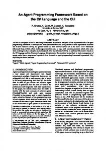
Fig. 1. An illustration of the proposed spectrum-sensing framework for an IEEE 802.22 WRAN. The BS selects an optimal set of sensors (black nodes) for distributed (or cooperative) sensing and determines the optimal stopping time for sensing in each CDT. At each QP, the BS collects the test statistics {tn }, i.e., RSSs, from sensors, compare them with the pre-established RSS profile and updates the decision statistic Λn . The BS schedules QPs until the Λn reaches one of the decision thresholds (see Section IV for details).

D. Outline of the Proposed Approach The performance of energy detection is highly susceptible to signal-to-noise ratio (SNR), thus hampering its applicability in a low SNR environment such as IEEE 802.22 WRANs and preventing efficient discovery of spectrum opportunities. To overcome this problem and design an efficient cooperative sensing algorithm, we exploit both the spatial and temporal variations of RSSs among collaborating sensors. In 802.22 WRANs, the RSS at each sensor is (pseudo) time-invariant due to the static deployment of the sensors (i.e., CPEs). Thus, the key idea is to allow the BS learn the RSS distributions at sensors and build the spatial RSS profile of them. Then, upon collecting the sensing results at each QP, the BS compares the observed RSS values with the RSS profile where similarity to the RSS distribution with primary signal can be interpreted as an indication of the presence of a primary signal, and vice versa. Using the RSS profile, the BS schedules QPs until it accumulates sufficient observations to decide whether or not a primary signal exists with a certain performance bound. Our proposed sensing framework consists of the following three components, which closely interact with each other: • Sensor selector that selects an optimal set of sensors for cooperative sensing by analyzing their contributions to the improvement of detectability and the increase of sensing overhead (see Section IV-B). • RSS profile manager that establishes and maintains the spatial RSS distributions among collaborating sensors in the presence and the absence of a primary signal (see Section III-A). • Primary signal detector that adaptively schedules sensing and determines the presence of a primary signal. It provides detection schemes based on one-time sensing (see Section III-B) and a sequence of measurements (see Section IV-A). Fig. 1 illustrates our proposed spectrum-sensing framework, where the BS directs an optimally-chosen set of sensors to perform sensing until a decision is made on the existence of a primary signal, using a sequence of reported RSS values.

A. Construction of a Spatial RSS Profile We propose to build a spatial profile (or signature) of RSS distributions at multiple sensor locations, which will be used as a main reference for primary signal (i.e., DTV signal) detection. Fig. 2 plots an example of spatio-temporal variations of the test statistics (i.e., T in Eq. (1)) at 15 sensors under log-normal shadow fading with σdB = 5.5. It clearly shows spatial diversity in RSSs along with their temporal variations due to measurement error.4 The BS can, therefore, learn the distribution of RSSs at each sensor location and combine them to construct a spatial RSS profile. For RSS profiling, we assume a large enough training period (including both ON/OFF periods of the primary transmitter) for accurate estimation of RSS distributions. Note that when no primary signal exists, i.e., OFF periods, each sensor estimates the noise power distribution for RSS profiling. Then, the measured RSS values during both ON and OFF periods are reported to the BS where the RSS profile is generated and stored for primary detection in future by comparing it with the observed RSS values. Recall that the distribution of test statistic, T (equivalent to the RSS), of the energy detector can be approximated as Gaussian (see Eq. (2)) using the CLT in both ON/OFF periods. Thus, the RSS profile of ns cooperating sensors is an ns -dimensional Gaussian distribution, the parameters of which can be easily estimated using well-known techniques, such as maximum-likelihood estimation (MLE). Let µk and Σk , k ∈ {0, 1}, denote the mean vector and the covariance matrix during ON(1)/OFF(0) periods. Since the RSS distributions at each sensor location are (pseudo) time-invariant (except the measurement error due to limited sensing time) due to static deployment of secondary users (i.e., CPEs), the RSS profile can be used reliably without frequently updating it. B. Detection with One-Time Sensing Based on Linear Discriminant Analysis (LDA) We now propose a detection rule using an RSS profile given a single sensing measurement. Let x = [T1 , . . . , Tns ]T denote the vector of test statistics (see Eq. (2)) of the energy detector measured by ns cooperating sensors. Our incumbent detection problem is then a binary Gaussian classification problem where the observed test statistic x ∈ Rns ×1 belongs to one of two classes, H0 or H1 , where H0 : x ∼ N (µ0 , Σ0 ) H1 : x ∼ N (µ1 , Σ1 )

(no primary signal) (primary signal exists),

where µk ∈ Rns ×1 and Σk ∈ Rns ×ns are the estimated mean vector and the covariance matrix of RSS distributions under Hk , respectively. Note that Σ0 = σn2 I where I is an ns × ns identity matrix and σn2 = (N B)2 /M . 4 The intensity of temporal RSS variations depends on the sensing time, i.e., M , in Eq. (1); the shorter the sensing time, the larger the temporal RSS variations due to the increase of measurement error.

−13

x 10 4.5

test statistics (T)

III. RSS-P ROFILE -BASED C OOPERATIVE S ENSING In this section, we first present the construction of a spatial RSS profile and formulate the primary detection based on one-time sensing as a binary classification problem. Then, we present the theoretical performance of detection performance under log-normal shadowing.

4 3.5 3 2.5 0 5

15 10

time

10 15

5 20

0

sensor index

Fig. 2. Example time sequences of test statistics {Ti } for 1 ≤ i ≤ 15 where PR = −110 dBm, N B = −95.2 dBm, M = 6 × 103 , and σdB = 5.5 dB. It clearly shows spatial and temporal variations in the test statistics.

In general, under the assumption of unequal covariance matrices, the optimal decision rule for our detection problem can be found via quadratic discriminant analysis (QDA) [22]. Although QDA provides an optimal decision rule for a general multivariate Gaussian with unequal covariance matrices, it does not yield a closed-form expression for the error probability because of its quadratic decision boundaries [23]. Interestingly, however, the quadratic decision rule can actually be linearized using a linear discriminant analysis (LDA) in our problem on the basis of the following two important observations, i.e., Σ1 can be: 1) assumed as an identity matrix with fixed sensor locations, and then, 2) approximated as Σ1 ≈ Σ0 = σn2 I in a very low SNR environment. Regarding the first observation, the covariance matrix Σ1 may not appear to be an identity matrix because of the existence of shadow correlation in primary signal strengths [24]. However, as mentioned earlier, when sensor locations are fixed, their RSS is also (pseudo) time-invariant and the randomness in the test statistics comes only from the noise processes (i.e., measurement errors), which are independent of each other. Thus, the correlation of RSSs between any pair of sensors is virtually 0, so we can assume that Σ1 is also an identity matrix as Σ0 . Regarding the second observation, the received primary signal strength P may be significantly lower than that of the noise power in a very low SNR environment of 802.22. For example, at the DTV signal detection threshold, i.e., −116 dBm, the SNR is less than −20 dB, assuming the typical noise level N B = −95.2 dBm [4]. Therefore, it is reasonable to assume that Pi +N B ≈ N B ∀i, and thus, Σ1 ≈ Σ0 = σn2 I. Fig. 3 justifies these assumptions by showing that the error performances of QDA and LDA are almost the same in very low SNR environments. Consequently, under the assumption of a common covariance matrix Σk = σn2 I ∀k, we have a simple distance-based decision rule for incumbent detection: H1 kx − µ0 k ≷ kx − µ1 k. H0

noise uncertainty (∆) = 0 dB, σdB = 5.5, ns = 10

1

D. Effect of Log-normal Shadowing We now study the effect of shadow fading on detection performance by investigating its impact on the distance kwk. Recall that w is defined as the difference in RSSs under both hypotheses, i.e., w = µ1 − µ0 = [P1 , . . . , Pns ]T . Therefore, based on Eq. (3), kwk under shadow fading is given as: X 1/2 X  ns ns
2 1/2 Pi2 = PR · , (7) kwkshadow = eYi

QDA LDA e

error probability (P )

0.8

0.6

0.4

0.2

i=1

0 −130

−125

−120

−115

−110

average received signal strength (P) (dBm)

Fig. 3. Error performances of QDA vs. LDA: the performance difference is insignificant in a very low SNR environment; note that the noise power is assumed to be −95.2 dBm. This is the results of a Monte Carlo simulation with 107 runs.

Clearly, the decision is made based solely on the distance between the observed RSS vector, x, and the mean vectors of the RSS profile, µk , under both hypotheses. Therefore, our RSS-profile based detection rule allows a simple data fusion at the BS, thus reducing the computational overhead, while outperforming the traditional threshold-based detection rules, e.g., the OR-rule (see Section V for detailed results). C. Theoretical Performance Let T (x) , wT x denote the test statistic for incumbent detection, which is calculated based on the observed RSS vector x, where w , (µ1 − µ0 ) ∈ Rns ×1 . Note that kwk is the Euclidean distance between the centroids of two Gaussian distributions under both hypotheses, where the centroids µi are the vectors of average RSSs at sensor locations. Then, it can be easily shown that the test statistic T (x) follows a Gaussian distribution, i.e., T (x) ∼ N wT µk , σn2 kwk2 ) under Hk ∀k. Then, the probability of false alarm under our LDA-based decision rule with the decision threshold η ∈ R is given as: PFLDA , P rob(T (x) > η | H0 ) A   η − wT µ0 , =Q σn kwk

where Q(·) is the Q-function. Using Eq. (4), the decision threshold η can be derived for the desired PFLDA as: A
−1 LDA T η = σn · kwk · Q PF A + w µ0 . (5) Then, based on Eqs. (4) and (5), the probability of miss LDA detection, PMD , is given as: LDA PMD , P rob(T (x) < η | H1 )  
kwk = 1 − Q Q−1 PFLDA − . A σn

To understand the impact of shadow fading on detection LDA performance (in terms of PMD given a fixed PFLDA A ), it is desirable to study the distribution of kwkshadow in Eq. (7). Unfortunately, there is no closed-form expression available for the power sum of log-normal random variables in Eq. (7) [25]. However, the power sum can be approximated accurately by rendering the′ sum itself as another log-normal random variable [26]. Let eZ ∼ e2Y1 + e2Y2 + · · · + e2Yns . Then, by following the result in [26], the sum can be approximated by matching Z′ its ′ mean and′ variance with e . The first two moments of 2 ′ 2 eZ are E[eZ ] = eµZ ′ +σZ ′ /2 and E[e2Z ] = e2µZ ′ +2σZ ′ . Our final goal is to approximate the square root of the power ′ sum, i.e., eZ = (eZ )1/2 , which is still a log-normal random ′ variable. Thus, by the first two moments of eZ′ and Pequating ns the power sum, i=1 (eYi )2 , and then taking eZ = (eZ )1/2 , we have kwkshadow ≈ PR · eZ with the random variable 2 eZ ∼ Log-N (µZ , σZ ) where:  4σ2  1 (e − 1) 2 σZ = log +1 , (9) 4 ns and

(4)

(6)

Eq. (6) indicates that, when the desired PFLDA is given, the A 2 LDA achievable PMD depends on the noise variance σn2 = (NMB) LDA and the distance kwk. That is, the PMD decreases as the sensing duration (thus the number M of samples) increases since a large number of samples would make the decision more accurate due to the reduced noise variance (measurement error). On the other hand, the distance kwk would be affected by the intensity of the shadow fading, as we discuss next.

i=1

where PR is the average RSS in the cell due to path loss. As mentioned earlier, Yi is a location-dependent realization of a random variable Y ∼ N (0, σ 2 ) where σ = 0.1 ln(10)σdB . Note that the AWGN channel can be regarded as a special case with no log-normal fading component, i.e., σdB = 0, and thus, kwk under AWGN channel is given as: √ kwkAW GN = PR · ns ∀ns ∈ N. (8)

1 σ2 log(ns ) + σ 2 − Z . (10) 2 4 Assuming that the sensors experience independent lognormal shadow fading, we can derive the average miss detection probability as:   Z ∞
PR · ez LDA −1 LDA P MD = 1−Q Q PF A − · fz · dz, σn −∞  2 Z) 1 where fz = σ √ exp − (z−µ , −∞ < z < ∞. 2 2σ 2π Z Z The simulation results (in Section V) show that LDAbased detection rule for one-time sensing significantly outperforms the traditional OR-rule in incumbent detection (see Section V-B). However, the results indicate that the detection requirement of 802.22 is guaranteed to be met only under certain conditions, e.g., shadow fading with a high dB-spread, even with cooperative sensing. Therefore, in what follows, we present an optimal cooperative sensing framework that is designed to: (i) select an optimal set of sensors and (ii) find an optimal stop time for sensing in each CDT, to further improve the detection performance with minimal sensing overhead. µZ =

IV. O PTIMAL C OOPERATIVE S ENSING F RAMEWORK FOR S ENSING OVERHEAD M INIMIZATION In this section, we first propose an adaptive online algorithm for sensing scheduling that finds an optimal stopping time for quiet periods (QPs) in a CDT, subject to the detection requirements of 802.22, assuming a set of collaborative sensors is given. We then present an algorithm for selecting an optimal set of sensors that minimizes the average sensing-time. A. Optimal Stopping Rule for Sensing Scheduling In the TSS mechanism in 802.22, fast-sensing (i.e., energy detection) is scheduled at discrete-time intervals,5 and thus the BS receives a sequence of observations (i.e., RSS vectors) from the sensors. This makes sequential detection suitable for our problem. In particular, among various sequential detection techniques, we adopt Wald’s Sequential Probability Ratio Test (SPRT) [27] since it is optimal in the sense of minimizing the average number of observations, given bounded probabilities of false alarm and miss detection. Let tn , σn−1 · kwk−1 · T (xn ) denote the normalized test statistic based on the observed RSS vector xn in the nth QP. Then, in SPRT, the decision is made based on the observed sequence of test statistics, {tn }N n=1 , using the following rule: ΛN ≥ B ⇒ accept H1 (primary signal exists) ΛN < A ⇒ accept H0 (no primary signal) A ≤ ΛN < B ⇒ take another observation,

where A and B (0 < A < B < ∞) are the detection thresholds that depend on the desired values of PF A and PMD . The decision statistic ΛN is the log-likelihood ratio based on N sequential observations (i.e., test statistics) t1 , . . . , tN as: ΛN , λ(t1 , . . . , tN ) = ln

f1 (t1 , . . . , tN ) , f0 (t1 , . . . , tN )

(11)

where fk (t1 , . . . , tN ) is the joint p.d.f. of the sequence of observations under hypotheses Hk ∀k. Recall that {tn }N n=1 are Gaussian, and w.o.l.g., we assume that they are i.i.d. Then, Eq. (11) becomes: ΛN =

N X

λn =

n=1

N X

n=1

ln

f1 (tn ) , f0 (tn )

(12) T

µk ∀k. where fk (tn ) is N (θk , 1) with θk , E[tn | Hk ] = σwn kwk Then, we have: f1 (tn ) 1 λn = ln = (θ1 − θ0 ) tn + (θ02 − θ12 ). (13) f0 (tn ) 2 Based on Eqs. (12) and (13), the decision statistic ΛN can be expressed as:

Algorithm 1 O NLINE S ENSING S CHEDULING At the beginning of a CDT period, the BS does the following 1: while each round n ∈ [1, Nmax ] of quiet period (QP) do 2: Receive results of energy detector (i.e., RSS) xn from sensors 3: tn ← σn−1 · kwk−1 · T (xn ) // Calculate test statistic 4: ΛN ← ΛN + (θ1 − θ0 ) tn + 12 (θ02 − θ12 ) 5: if ΛN ≥ B then 6: A primary exists and we schedule fine-sensing (or initiate 7: 8: 9: 10: 11: 12: 13: 14:

the channel vacation procedure) else if ΛN < A then A primary does not exist and we defer QP until the beginning of next CDT period else if n = Nmax then Schedule fine-sensing for in-depth measurement else Schedule another QP and wait for the observation end if end while

and the actual achievable error probabilities, denoted as α and β, have the following relationships: β∗ α∗ , β≤ , and α + β ≤ α∗ + β ∗ . (16) ∗ 1−β 1 − α∗ Eq. (16) indicates that the actual achievable error probabilities, i.e., α and β, can only be slightly larger than the desired values α∗ and β ∗ . For example, with the desired values of α∗ = β ∗ = 0.1, the actual values α and β will be no larger than 0.111. Recall that our goal is to minimize the number of times the spectrum needs to be sensed, with the decision thresholds derived from the target detection probabilities as shown in Eq. (15). We therefore consider the number of QPs until a decision is made (i.e., either the boundary A or B is reached) as our main performance metric. The average number of QPs, E[N ], required for decision-making can be computed as: α≤

E[ΛN ] = E[N ] × E[λ | Hk ].

First, using Eq. (13), the average value of λ under Hk can be derived as: 1 E[λ | Hk ] = (θ1 − θ0 ) θk + (θ02 − θ12 ). (18) 2 The average of ΛN can then be found as follows. Suppose H0 holds, then ΛN will reach B (i.e., false alarm) with the desired false alarm probability α∗ ; otherwise, it will reach A. Thus, using Eq. (15), we have: 1 − β∗ β∗ + (1 − α∗ ) ln . (19) ∗ α 1 − α∗ Based on Eqs. (17), (18) and (19), we can derive the average required QPs for decision-making as: E[ΛN | H0 ] = α∗ ln

∗

ΛN

N X

N = (θ1 − θ0 ) tn + (θ02 − θ12 ). 2 n=1

(14)

Let α∗ and β ∗ denote the desired values of PF A and PMD , respectively. Then, the decision boundaries are given by [27]: β∗ 1 − β∗ A = ln and B = ln , (15) ∗ 1−α α∗ 5 In

IEEE 802.22, the interval between consecutive QPs must be separated by at least 10 ms, i.e., one MAC frame size [15].

(17)

E[N | H0 ] =

∗

β ∗ α∗ ln 1−β α∗ + (1 − α ) ln 1−α∗

(θ1 − θ0 ) θ0 + 12 (θ02 − θ12 )

.

(20)

.

(21)

Similarly, we can derive:

∗

E[N | H1 ] =

∗

β ∗ (1 − β ∗ ) ln 1−β α∗ + β ln 1−α∗

(θ1 − θ0 ) θ1 + 12 (θ02 − θ12 )

Based on Eqs. (11)–(21), Algorithm 1 describes our online algorithm for scheduling QPs that finds an optimal stopping time for sensing.

In addition to the detection-accuracy requirements in terms of PF A and PMD , 802.22 also has a timing requirement on primary detection, i.e., CDT. Thus, our scheduling algorithm should allow the BS to make a fast decision (i.e, reach one of the boundaries) within a CDT, thus eliminating the need for expensive feature detection; otherwise, the BS needs to schedule a fine-sensing period at the end of the CDT. However, in practice, the maximum number of QPs, Nmax , that can be scheduled within a CDT is constrained by several factors, such as inter-sensing interval, initial sensing delay, sensing time, and length of a CDT [21]. Therefore, we set a threshold Pth , a design parameter, such that the BS must reach a conclusion within Nmax QPs with probability greater than or equal to the Pth . Let Nopt denote the optimal stopping time of QPs with Algorithm 1. Then, we are interested in deriving the probability that Nopt ≤ Nmax , which should be no less than Pth . Although an approximate formula for the distribution of Nopt can be derived, we instead derive a lower limit on the probability for computational efficiency [27]. Suppose ΛNmax ≥ B. Then we have Nopt ≤ Nmax , and thus, the following inequality holds:
P rob Nopt ≤ Nmax ) ≥ P rob(ΛNmax ≥ B . (22)

Since Nmax is sufficiently large in practice, we can use the central limit theorem (CLT), and then the inequality ΛNmax ≥ B can be written as: ΛNmax − Nmax E[λ | H1 ] B − Nmax E[λ | H1 ] √ √ ≥ , (23) Nmax σ1 (λ) Nmax σ1 (λ)

where σ1 (λ) is the standard deviation of λ under H1 , which can be derived as σk (λ) = (θ1 − θ0 ) ∀k from Eq. (13). Then, the left-hand side of Eq. (23) is normally distributed with zero mean and unit variance when H1 is true. Therefore, based on Eqs. (22) and (23), we have the following lower bound on the probability that the BS makes a decision within Nmax observations (i.e, QPs): !
B − Nmax E[λ | H1 ] √ P rob Nopt ≤ Nmax ≥ Q . (24) Nmax σ1 (λ) This lower bound will be considered in our algorithm for selecting an optimal set of sensors as described next.

B. Algorithm for Selecting an Optimal Set of Sensors We now turn to the problem of finding the best set of sensors that minimizes the total sensing overhead. Let Φ denote the total set of sensors available for cooperative sensing with estimated RSS distributions via training. The idea is to utilize a subset Ω ⊆ Φ of sensors with relatively high average RSS values (e.g., those located close to the primary transmitter or outside a deep fading area), thus minimizing both the number of cooperating sensors and the number of QPs in incumbent detection, while guaranteeing the detectability requirements. Given a subset of sensors, Ω, the total expected sensing overhead within a CDT can be expressed as: n o O(Ω) = min E[N (Ω)], Nmax × TD (Ω), (25)

where TD (Ω) is the total time duration for a single sensing, which consists of a QP and a measurement reporting period: TD (Ω) = QP + |Ω| × TR ,

(26)

Algorithm 2 S ELECTION OF AN O PTIMAL S ET OF S ENSORS 1: 2: 3: 4: 5: 6: 7: 8: 9: 10: 11: 12: 13: 14: 15: 16: 17:

Initialize the desired detection parameters PF A ,PM D ,Pth Initialize the set of available sensors Φ = {χ1 , . . . , χns } Initialize the optimal set of sensors Ω∗ ← ∅ Initialize the sensing overhead O∗ ← ∞ while Φ 6= ∅ do χ∗ ← arg maxχi ∈Φ {Pi } // Pi = PR · eYi Φ ← Φ \ {χ∗ } Ω ← Ω∗ ∪ {χ∗ } N ∗ ← min{E[N (Ω, PF A , PM D )], Nmax } O ← N ∗ × TD (Ω) if O > O∗ and P rob(Nopt ≤ Nmax ) ≥ Pth then return Ω∗ else Ω∗ ← Ω O∗ ← O end if end while

where TR is the duration of a time-slot for reporting the sensing result to the BS. Then, based on Eqs. (24), (25), and (26), our problem of finding an optimal set of sensors can be formally stated as: Find

Ω∗ = arg min O(Ω) Ω⊆Φ

subject to P rob(Nopt ≤ Nmax ) ≥ Pth . For this, we propose a simple algorithm as described in Algorithm 2. The idea is that we sort the sensors in descending order of averge RSS (i.e., Pi ) and then add sensors to Ω from the top of the list until the total sensing overhead increases by adding another sensor, and the detection constraint (i.e., Pth ) is satisfied (line 11). The algorithm provides an optimal solution with a low computational overhead, i.e., O(|Φ|), while the exhaustive search requires O(2|Φ| −1). The algorithm is shown to reduce the sensing overhead significantly (see Section V-C), while guaranteeing the detectability requirements of 802.22. V. P ERFORMANCE E VALUATION This section evaluates the proposed algorithms using MATLAB-based simulation. These algorithms are comparatively evaluated against the OR-rule under various fading conditions. A. Simulation Setup We consider the IEEE 802.22 WRAN environment with a single primary transmitter (i.e., TV transmitter) and multiple secondary users (i.e., CPEs) located at the edge of the keep-out radius (i.e., 150.3 km) where the average received strength of a TV signal is below −96.5 dBm [20]. We use the commonlyused noise power (N B)i = −95.2 ± ∆i dBm [4], where ∆i is the noise uncertainty (in dB) at sensor i and B is the channel bandwidth, i.e., 6 MHz. We consider shadow fading with various dB-spreads σdB = 0, 2, 5.5 (dB); while σdB = 5.5 dB is typical in 802.22 [20], it can vary depending on local environments, e.g., distance/angle to the BS [28]. Throughout the simulation, we assume 10 cooperating sensors unless specified otherwise, and the time-slot duration for reporting a RSS measurement (TR ) is fixed at 0.2 ms. For RSS profiling, 104 samples were used for estimating the RSS distributions, which consumes only 10 seconds of total sensing time. The

noise uncertainty (∆) = 0 dB, TS = 1 ms, PFA=0.1, ns=10 DTV signal detection threshold

dB dB

FA

s

SNR wall 0.6

LDA, σdB=5.5

0.4

LDA, σdB=5.5

0.8

dB

LDA, AWGN LDA, σdB=2

P

PMD

dB

LDA, AWGN LDA, σdB=2

OR, σ =5.5

0.6

dB

LDA, σ =5.5

PMD

S

1

OR, AWGN OR, σdB=2

LDA, AWGN LDA, σ =2

0.6

i

0.8

OR, σ =5.5

0.8

∆ ~ N(0,1) dB, T = 1 ms, P =0.1, n = 10

noise uncertainty (∆) = 0 dB, TS = 1 ms, PFA=0.1, PR=−116 dBm

OR, AWGN OR, σ =2

MD

1

0.4

0.4

0.2 0.2

0.2

0 −135

−130

−125

−120

−115

−110

0 1

−105

5

average received signal strength (PR) (dBm)

10

15

0 −125

20

(a) Effect of shadow fading

−120

−115

−110

−105

−100

−95

average received signal strength (P ) (dBm)

number of sensors (ns)

R

(b) Effect of number of cooperating sensors

(c) Effect of noise uncertainty

Fig. 4. Performance of LDA-based detection rule for one-time sensing. The figures show that LDA-based detection (a) outperforms the OR-rule in all fading environments, (b) better exploits shadow fading via cooperative sensing, and (c) successfully overcomes noise uncertainty.

20

TS = 2 ms T = 5 ms S

15

10

5

0

−125

−124

−123

−122

−121

average received signal strength (PR) (dBm)

Fig. 5. Effect of sensing duration (TS ) on average number of QPs. The larger the sensing duration, the more accurate the sensing result, thus reducing the number of QPs needed.

noise uncertainty (∆) = 0 dB, TS = 1 ms, PFA=PMD=0.1, ns=10

n.u. (∆) = 0 dB, T = 1 ms, P =P

100

OR, AWGN OR, σ =2 dB

80

OR, σ =5.5 dB

SPRT, AWGN SPRT, σ =2

60

dB

SPRT, σdB=5.5

40

20

0 −130

−125

−120

−115

−110

average received signal strength (P ) (dBm) R

Fig. 6. Average number of QPs scheduled to meet the detectability requirement of 802.22. Our online sensing scheduling algorithm lowers the sensor’s operating range (feasible RSS region) by 13 dB.

performance of the proposed algorithms are evaluated under various shadow fading conditions and compared with OR-rulebased cooperative sensing algorithms. B. Performance of LDA-based Detection Scheme for OneTime Sensing We first evaluate the performance of proposed LDA-based detection scheme for one-time sensing under various fading conditions. We assume that the sensors are randomly selected. 1) Effects of Shadow Fading (σdB ): Fig. 4(a) shows that our LDA-based detection significantly outperforms the ORrule in all simulated scenarios, thanks to its ability to set the near-optimal detection threshold (i.e., an (ns − 1)-dimensional hyperplane) based on the spatial RSS profile; the OR-rule, in contrast, uses the same threshold at all sensors for simplicity [3], [7]. Interestingly, both detection schemes perform better as shadow fading becomes more intense (i.e., higher σdB ) at a given average primary signal strength. This is because of the heavy-tailed distribution of the primary signal strength, due to log-normally-distributed shadow fading [29]. Therefore, a large dB-spread, σdB , improves detection performance, especially in a low SNR environment. 2) Effects of Number of Sensors (ns ): We now study the impact of number of sensors on detection performance. We set the average signal strength (PR ) to the DTV signal detection threshold (i.e., −116 dBm). Fig. 4(b) shows that the LDAbased detection outperforms the OR-rule-based detection and

S

20

sensing−time overhead (%)

TS = 1 ms

average number of sensings (N)

average number of sensings (N)

noise uncertainty (∆) = 0 dB, PFA=PMD=0.1, σdB=5.5

15

FA

=0.1, σ =5.5, P =0.9

MD

dB

th

SS, |Φ|=10 SS, |Φ|=20 SS, |Φ|=50 w/o SS, |Φ|=10 w/o SS, |Φ|=20 w/o SS, |Φ|=50

w/o sensor selection

sensor selection

10

5

0 −130

−129

−128

−127

−126

−125

−124

average received signal strength (P ) (dBm) R

Fig. 7. Performance of the optimal sensor selection algorithm. Our proposed sensor selection algorithm reduces sensing overhead significantly over the algorithm without sensor selection.

the performance gap increases as the number of cooperating sensors increases. This is because, in the LDA-based detection, all the sensors contribute to the enhancement of the detection performance via RSS-profile, thus fully exploiting spatial RSS diversity, whereas, in the OR-rule, only a few sensors with high RSSs (e.g., above the detection threshold) contribute to the detection of a primary signal. 3) Effects of Noise Uncertainty (∆): The noise uncertainty is one of the main obstacles in using the energy detection in a very low SNR environment such as 802.22 [30]. We assume that the noise uncertainty at sensor i is i.i.d. Gaussian random variable with 1 dB variance, i.e., ∆i ∼ N (0, 1) ∀i. Fig. 4(c) shows the average PMD obtained by 104 runs of Monte Carlo tests. In the tests, the decision thresholds are adjusted so that the average PF A remains below 0.1. Note that, when the OR-rule is employed, the detector completely fails below SN Rwall (under AWGN channel), which is −98.5 dBm when ∆i = 1 dB ∀i.6 The figure, however, shows that under the practical assumption that the noise uncertainty is independent at the sensors, the LDA-based detection works well below SN Rwall even with a one-time sensing and performs better as shadow fading becomes more intense, i.e., higher σdB , thanks to its ability to exploit spatial RSS diversity. 6 This is a reasonable assumption since noise uncertainty can be bounded by ±1 (dB) considering several contributing factors such as calibration error, thermal noise variation, changes in LNA amplifier gain, etc. [31].

C. Performance of Online Sensing Scheduling with Optimal Selection of Sensors We now evaluate the performance of the proposed online sensing scheduling and optimal sensor-selection algorithms. 1) Effects of Sensing Time (TS ): Fig. 5 plots the average number of QPs required to make a final decision as well as the interval (−0.5 σTS , +0.5 σTS ). As expected, as we increase the sensing time, the average number of QPs decreases in all simulated scenarios. This is because the more samples the detector have, the more accurate the sensing results, thus eliminating ambiguity on the existence of a primary signal. Clearly, there is a tradeoff between the sensing time (TS ) and the number of QPs (N ) in our sensing scheduling, which is part of our future work. 2) Impact on QP Minimization (N ): Here we study the performance of our online sensing scheduling algorithm that finds an optimal stopping time for scheduling QPs. We assume that the maximum number Nmax of QPs that can be scheduled in a CDT is 100. Fig. 6 shows that our online sensing scheduling algorithm significantly reduces the average number of QPs compared to the OR-rule-based scheduling scheme, due to its ability to find the optimal stopping time for scheduling QPs, instead of scheduling a fixed number of QPs as the OR-rule-based approach. As a result, our algorithm expands the feasible region of the energy detector’s operation significantly. For example, the scheduling threshold under the shadow fading with σdB = 5.5 is as low as −129.5 dBm with our proposed algorithm, whereas it is −116 dBm with the ORrule. Interestingly, in the OR-rule, there is almost no benefit from scheduling QPs because RSSs do not change over time (except the measurement errors) at fixed sensor locations. 3) Impact on Sensing Overhead (O): We now demonstrate the performance of our optimal sensor-selection algorithm in terms of the reduction of sensing overhead. The sensing overhead here is defined as the average fraction of time spent on sensing within a CDT period (see Eq. (25)). Fig. 7 compares the average sensing overhead of a cooperative sensing with sensor selection (denoted as SS) against the one without sensor selection. The figure shows that our algorithm minimizes the average sensing overhead significantly because it selects only a subset of sensors with high average RSSs, thus minimizing both the number of QPs and the sensing result reporting time. VI. C ONCLUSION In this paper, we proposed an optimal spectrum sensing framework for IEEE 802.22 WRANs that minimizes the average sensing-time, while guaranteeing the performance requirement of IEEE 802.22 to be met. We exploit the spatiotemporal variations in received primary signal strengths for our cooperative sensing that consists of (i) RSS-profile manager that learns the spatial RSS distribution among sensors, (ii) sensor selector that selects an optimal set of sensors by making a tradeoff between sensor capability and sensing overhead, and (iii) primary signal detector that uses the RSS-profile to provide a simple linear decision rule for one-time sensing, and optimal stopping time for scheduling of sensing periods. Our evaluation results show that the proposed sensing algorithms ensure the detection requirements of 802.22, while minimizing the sensing overhead significantly.

R EFERENCES [1] IEEE 802.22 Working Group on Wireless Regional Area Networks, http://www.ieee802.org/22/. [2] C. Cordeiro, K. Challapali, D. Birru, and S. Shankar, “IEEE 802.22: An Introduction to the First Wireless Standard based on Cognitive Radio,” Journal of Communications, vol. 1, no. 1, pp. 38–47, April 2006. [3] S. Shellhammer, S. Shankar, R. Tandra, and J. Tomcik, “Performance of Power Detector Sensors of DTV Signals in IEEE 802.22 WRANs,” in ACM TAPAS ’06, Aug 2006. [4] S. Shellhammer and R. Tandra, “Performance of the Power Detector with Noise Uncertainty,” IEEE 802.22-06/0134r0, July 2006. [5] ——, “An Evaluation of DTV Pilot Power Detection,” IEEE 802.2206/0188r0, Sep 2006. [6] D. Cabric, S. M. Mishra, and R. W. Brodersen, “Implementation Issues in Spectrum Sensing for Cognitive Radios,” in Asilomar conference on Signals, Systems and Computers ’04, Nov 2004, pp. 772–776. [7] A. Ghasemi and E. S. Sousa, “Collaborative Spectrum Sensing for Opportunistic Access in Fading Environments,” in IEEE DySPAN ’05, Nov 2005, pp. 131–136. [8] E. Visotsky, S. Kuffner, and R. Peterson, “On Collaborative Detection of TV Transmissions in Support of Dynamic Spectrum Sharing,” in IEEE DySPAN ’05, Nov 2005, pp. 338–345. [9] A. Ghasemi and E. S. Sousa, “Opportunistic Spectrum Access in Fading Channels Through Collaborative Sensing,” Journal of Communications, vol. 2, no. 2, pp. 71–82, March 2007. [10] S. M. Mishra, A. Sahai, and R. W. Brodersen, “Cooperative Sensing among Cognitive Radios,” in IEEE ICC ’06, June 2006, pp. 1658–1663. [11] J. Unnikrishnan and V. V. Veeravalli, “Cooperative Sensing for Primary Detection in Cognitive Radio,” IEEE Journal of Selected Topics in Signal Processing, vol. 2, no. 1, pp. 18–27, Feb 2008. [12] G. Chouinard, “Use of Collaborative Sensing to Reduce False Positive Results,” IEEE 802.22-08/0118r0, May 2008. [13] Y. Sel´en, H. Tullberg, and J. Kronander, “Sensor Selection for Cooperative Spectrum Sensing,” in IEEE DySPAN ’08, Oct 2008. [14] H. Kim and K. G. Shin, “In-band Spectrum Sensing in Cognitive Radio Networks: Energy Detection or Feature Detection?” in ACM MobiCom ’08, Sep 2008, pp. 14–25. [15] D. Cavalcanti and C. Cordeiro, “Proposed Resolution for Comments Related to the Superframe and Sensing,” IEEE 802.22-07/0176r0, April 2007. [16] W.-Y. Lee and I. F. Akyildiz, “Optimal Spectrum Sensing Framework for Cognitive Radio Networks,” IEEE Transactions on Wireless Communications, vol. 7, no. 10, pp. 3845–3857, Oct 2008. [17] S. Huang, X. Liu, and Z. Ding, “Optimal Sensing-Transmission Structure for Dynamic Spectrum Access,” in IEEE INFOCOM ’09, April 2009. [18] J. Benko et al., “Draft PHY/MAC Specification for IEEE 802.22,” IEEE 802.22-06/0069r1, May 2006. [19] S. Shellhammer, “Performance of the Power Detector,” IEEE 802.2206/0075r0, May 2006. [20] S. Shellhammer, V. Tawil, G. Chouinard, M. Muterspaugh, and M. Ghosh, “Spectrum Sensing Simulation Model,” IEEE 802.2206/0028r10, Sep 2006. [21] S. Shellhammer and R. Tandra, “Numerical Spectrum Sensing Requirements,” IEEE 802.22-06/0088r0, June 2006. [22] T. Hastie, R. Tibshirani, and J. Friedman, The Elements of Statistical Learning. Springer, 2001. [23] M. M. E. Ayadi, M. S. Kamel, and F. Karray, “Toward a tight upper bound for the error probability of the binary Gaussian classification problem,” Pattern Recognition, vol. 41, no. 6, pp. 2120–2132, June 2008. [24] M. Gudmundson, “Correlation Model for Shadow Fading in Mobile Radio Systems,” Electronic Letters, vol. 27, no. 23, pp. 2145–2146, Nov 1991. [25] A. Safak, “Statistical Analysis of the Power Sum of Multiple Correlated Log-Normal Components,” IEEE Transactions on Vehicular Technology, vol. 42, no. 1, pp. 58–61, Feb 1993. [26] L. F. Fenton, “The Sum of Log-Normal Probability Distributions in Scatter Transmission Systems,” IRE Transactions on Communications Systems, vol. 8, no. 1, pp. 57–67, March 1960. [27] A. Wald, Sequential Analysis. Dover Publications, 2004. [28] Dean Kitchener et al., “Correlated Lognormal Shadowing Model,” IEEE C802.16j-06/059, July 2006. [29] T. Muetze, P. Stuedi, F. Kuhn, and G. Alonso, “Understanding Radio Irregularity in Wireless Networks,” in IEEE SECON ’08, June 2008, pp. 82–90. [30] R. Tandra and A. Sahai, “Fundamental limits on detection in low SNR under noise uncertainty,” in WirelessCom ’05, June 2005, pp. 464–469. [31] S. Shellhammer and G. Chouinard, “Spectrum Sensing Requirements Summary,” IEEE 802.22-06/0089r5, July 2006.