Proceedings of the 2007 American Control Conference Marriott Marquis Hotel at Times Square New York City, USA, July 11-13, 2007
FrA19.4
An Optimization Approach Based on Genetic Algorithm for Modeling Benson Type Boiler A. Ghaffari, A. Chaibakhsh and H. Parsa
Abstract — In this paper based on the fundamental laws of physics, thermodynamics principles and energy semiempirical laws for heat transfer, the mathematical models are developed and applied to electrical power generating plants in order to characterize the essential dynamic behavior of the boiler subsystems. These models are developed for a sub-critical once-through Benson type boiler based on the experimental data obtained in field experiments. An optimization approach based on genetic algorithm (GA) is executed to estimate the model parameters and fit the models response on the real system dynamics. Comparison between the responses of the corresponding models with the response of the real plants validates the accuracy and performance of modeling approach.
I
I. INTRODUCTION
ncreasing demand for electricity and growing need for more and safer power generating has motivated investigation into dynamic analysis of power plants to design more reliable control systems. Adequate information about the system dynamics is a key to design the suitable controllers. Better system performance means increase in power generation efficiency and decrease in the maintenance costs. The dynamics of most power plants are highly nonlinear with numerous uncertainties. Thus, no mathematical model can exactly describe such a complicated physical process, and there will always be modeling errors due to un-modeled dynamics and parametric uncertainties [1]. In order to characterize the essential dynamic behavior of power plants with representation of plant components, detailed models are needed [2]. Besides, detailed modeling of plants dynamics is often not efficient for control synthesis. There are complicated models based on finite element approximations to partial differential equations. These models are in the form of large simulation codes for plant design, simulators and commissioning. However, they are not normally used in control design approach because of their complexity [3]. The plant model should describe the plant dynamics with sufficient accuracy and not describe the microscopic details occurring within individual plant components [1].
Manuscript received September 14, 2006. A. Ghaffari is professor of Mechanical Engineering at K.N. Toosi University of Technology, Tehran, Iran (corresponding author to provide phone: 98-21-77-334-024; fax: +98-21-77-334-338). (E-mail:
[email protected]). A. Chaibakhsh is Ph.D. student of Mechanical Engineering at K.N. Toosi University of Technology, Tehran, Iran. (E-mail:
[email protected]). H. Parsa is Ph.D. student of Mechanical Engineering at Stevens Institute of Technology, Hoboken, NJ, USA, (E-mail:
[email protected]).
1-4244-0989-6/07/$25.00 ©2007 IEEE.
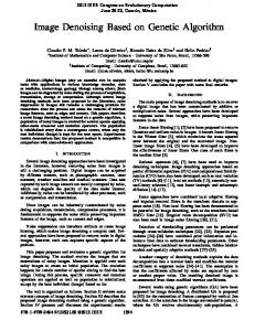
The analytical plant model can be formulated based on the fundamental laws of physics such as mass conservation, momentum, and energy semi-empirical laws for heat transfer and thermodynamics state conversion [3]. To build such analytical models, it is necessary to define their parameters with respect to boundaries, inputs, and outputs. Generally, the developed models need to be tuned by performing tests to validate for steady state and transient responses [4] [5]. When the identified model is nonlinear in the parameters, using conventional methods like standard least squares technique will not provide superior results. In these cases, evolutionary algorithm based methodologies are investigated as potential solutions to obtain good estimation of the model parameters [6]. Genetic algorithms have an advantage that it does not require a complete system model and can be employed to globally search for the optimal solution [7]. In this paper, the mathematical models with unknown parameters for subsystems of a once-through Benson type boiler are first developed based on the thermodynamics principles and energy balance. Then the related parameters are either determined from constructional data such as fuel and water steam specification, or by applying genetic algorithm (GA) techniques on the experimental data. Finally, the responses of the corresponding models are compared with the responses of the real plant in order to validate the accuracy and performance of the models. II. SYSTEM DESCRIPTION A 440 MW unit is considered for identification and modeling approach. The steam generator of a sub-critical once through Benson boiler with a steam mass rate of 1408 ton per hour is shown in Fig. (1). A single furnace with 14 bottom burners serves to heat all sections of the boiler. The hot water is converted to steam in evaporator, and is superheated by passing through superheaters. The evaporator outlet temperature is about 365 o C . The superheater consists of four sections built in the boiler second pass. The heating surface of superheater #1 is located in the boiler walls and is jointed to the superheater #2. The outlet steam temperature from these sections is about 407 o C . The steam leaves superheater #2 toward superheater #3. For rapid steam temperature control, four spray attemperators are located between the two sections. The outlet temperature should be kept constant at 470 o C . The steam for final superheating stage goes to superheater #4. The temperature at outlet header of this part should be constant at 535 o C . At the full load condition, the outlet superheated steam pressure is 18.1 MPa at the boiler outlet header. The superheated steam from main steam header is fed towards the high pressure (HP) turbine, and from high pressure turbine is discharged into the cold reheated
4860
FrA19.4
header. The steam temperature in cold reheat line is 351 o C . The outlet reheated steam temperature after RH-A should be constant at 452 o C and for RH-B should be constant at 535 o C . Also, at the full load condition, the outlet reheated steam pressure is 4.35 MPa .
and we have; dh ∂h dT (6) = dt ∂T dt By the additional simplification, for the superheater parts we have; dρ dT d hs .Vs s + ma .C p .Ta + ρ s .Vs .C p out (7) dt dt dt = Q + C p m& inTin − C p m& out Tout
[
It is shown that for the drum boiler, the changes in energy content of the water and metal masses are the physical phenomena that dominate the dynamics of the boiler [3]. The simulation results of models with detailed representation of temperature distribution show that by removing these terms, there is an off-set between the model response and the experimental data at the steady state conditions. To take these terms into account and to make the model response close to the response of the real plant, the related systems are expressed as a function of mass flow rates; dρ d (8) ma .C p .Ta = f (m& in ) u s .Vs s + dt dt
[
Fig. 1. Boiler Cross Section
III.
MODEL DEVELOPMENT
The boiler system can be decomposed into smaller components that can be analyzed and modeled separately. The behavior of the subsystems can be captured in terms of the balance equations and constructive equations [2] [3]. The steam-generating unit consists of economizer, evaporator, superheaters and reheater. In the boiler sections, the heat released by fuel combustion is transferred to the working fluid in the boiler. According to the global mass and energy balances, we have. d (1) [ρ s .Vs + ρ w .Vw ] = m& f − m& s dt d ρ s .u s .Vs + ρ w .u w .Vw + ma .C p .Ta ( 2) dt
[
]
= Q + m& f h f − m& s hs The right hand side of Eq. (2) represents the energy flow to the system from fuel and feed water and the energy flow from the system via the steam. Since the internal energy is u = h − p / ρ , the global energy balance can be written as; d ρ s .hs .Vs + ρ w .hw .Vw − pV + ma .C p .Ta (3) dt = Q + m& f h f − m& s hs Multiplying Eq. (1) by hw and subtracting the result from Eq. (3) we have, dρ dh dh (hs − hw ) Vs s + ρ s .Vs s + ρ w .Vw w dt dt dt d dp ( 4) + = Q + m& f (hw − h f ) ma .C p .Ta − V dt dt − m& s (hs − hw ) Where, ∂u ∂h (5) C p = , Cv = ∂T P ∂T v
[
]
[
]
]
]
This linear approximation is good enough to fit the model response to the real system response. (9) f (m& in ) = k1 . m& in Therefore, the equation (7) is captured as follow; dTout 1 = Q dt ρ s .Vs .C p 1 424 3
(10)
k2
+
1
ρ s .Vs
123
k m& in (Tin − Tout + 1
Cp
) + k0
k1
This equation is rewritten as follow; dTout (11) = K 2 (C p Q + m& in (Tin − Tout + B1 ) + B2 ) dt where 1 , B1 = k1 , B2 = k 0 ρ s .Vs (12) K2 = ρ s .Vs Cp The heat flow can be derived by using calorific value / lower heating value ( H v ) of the fuel. (13) Q = H v .m& fuel By considering K1 = H v .C p , the superheater model is derived; dTout (14) = K 2 ( K1m& fuel + m& in (Tin − Tout + B1 ) + B2 ) dt The dynamic behavior of the heated surfaces of the risers in the drum type boiler is shown in reference [3]. In the same way, these relations can be used to obtain the dynamics of steam generator. The specific internal energy for the steam and water mixture is, (15) h = α . hs + (1 − α ). hw where α is the mixture quality. The mass and energy balances for the heated surfaces are ∂ρ ∂ q ∂ρ h 1 ∂ q h Q (16) A + =0 , + = ∂t ∂ z ∂t A ∂z V
4861
FrA19.4
In the steady state condition, it is shown that the quality of mixture can be obtained, Q Az (17) α= q hc V The simulation results show that the steam quality can be expressed as a linear function of the fuel flow rate as follow, (19) α = f (m& fuel ) = K 3 .m& fuel With respect to these equations, the proposed temperature model for the evaporator and superheater sections are presented in Fig. (2) and Fig. (3). It should be noted that only the steam phase is presented in the superheater sections.
pressure loss is about 6 MPa . The main pressure drop is observed where vaporization takes place. In the steam side, the pressure loss due to change in flow velocity is prevailing. So, by neglecting the other effects, the pressure loss model can be captured based on the steam areas effect. The mass of accumulative volume is,
dM = m& in − m& out dt
(20)
The total accumulative action of any control volume in boiler consists of accumulative action of steam, hot liquid and metal parts. Therefore, differential equation for the total accumulative action can be written as follows.
∂M ∂M PS ∂M PW ∂M PM = + + ∂P ∂P ∂P ∂P
(21)
Noting that the effects of second and third terms on the right hand side of Eq. (21), comparing with the first term, are negligible. We have,
∂M ∂M PS = ∂P ∂P
(22)
In this sliding pressure Benson type boiler, the pressure differences are the driving forces for mass flow through the components. The change of steam mass due to the pressure change is given by,
dM d 1 =V. dP dP v( P)
(23)
By considering the value of polytrophic exponent is nearly 1.0 ( p.v = p0 .v0 ), If
dM >0 dP
for
dP > 0
(24)
From Eqs. (20) to (24), the outlet pressure is obtained;
P dP = 0 (m& in − m& out ) dt τ .mv
Fig. 2. Temperature Model for the Evaporator Section
(25)
This equation can be used as a general relation for pressure drop between turbine stages. A model for the mass flow responding to steam pressure changes is proposed by Borsi [7]. The swing of main steam flow strictly relies on the change of steam pressure.
dm& out m& out dP = dt 2( Pin 0 − Pout 0 ) dt
(26)
The superheater and reheater temperatures must be kept constant at specific temperature. The spray attemperators is implemented between these sections to control outlet temperature. Fig. 3. Temperature Model for the Superheater Sections
It should be noted that for modeling the boiler subsystems, the delay time is needed to be considered. This delay time is defined as the time required for burning the fuel in the furnace, transferring the released heat and absorbing transferred heat by fluid in boiler subsystems. The delay time is an important factor that affects the dynamics of boiler. The delay times of boiler subsystems are presented in Table (1) [Appendix]. Next, the outlet pressure of the boiler can be calculated based on the fluid dynamics principles. Naturally, the steam pressure will drop by passing through the boiler sections such that in the HP section of this boiler, the
4862
Fig. 4. Mass Flow- Pressure Model
FrA19.4
Furthermore, de-superheating spray is used to achieve mixing between the superheated steam at the outlet of the preceding component (e.g., the primary superheater). The water spray is modulated by suitable valves. Because the attemperator has a relatively small volume, the mass storage inside that is negligible. Therefore, the steadystate mass and energy balances yield
m& in + m& spray = m& out
(27)
m& in hin + m& spray hspary = m& out hout
(28)
data, is shown in Fig. (5). Therefore, Eq. (31) is solved for these unknown parameters at three steady state conditions. By solving these three set of linear equations, we obtain the initial values of parameters used in the model training process.
During a normal operation, steam flow m& out in the secondary superheater is imposed (over a wide band) by the load controller, the specific enthalpy hin is determined by upstream superheater and hspary is nearly constant. The inlet temperature of the second superheater, Tout is governed by the following equation [2].
(h − h ) 1 T&out = ∆hout = in out m& out C p mout Cp (hin − hspray ) m m& spray + in T&in − mout C p mout
(29) Fig. 5. The Actual Power Output at Four Diffrent Setpoints Between 195 to 440 MW.
This completes the dynamics modeling of different boiler subsystems. IV. PARAMETER ADJUSTMENT BY GENETIC ALGORITHM In this section, the parameters of the developed models are evaluated and adjusted by using genetic algorithm (GA) training approach. Genetic algorithm is specifically useful for those systems working under different operating conditions with different behavior. The GA determines the multiple next searching points using the evaluation values of multiple current searching points. The next searching points are determined by using the fitness values of the current searching points which are widely spread throughout the searching space. In conventional optimization methods, like gradient methods, in some cases the gradient information causes searching being trapped at a local minima point. The GA has the mutation operator to escape from these possible trapping points. These advantages cause that GA is preferred to other methods. For GA training, the error E is given by the mean value of squared difference between the target output y* and actual output y as follows;
E=
1 P * ∑ ( y p − y ( p) )2 P p=1
(30)
where P is the number of entries used for training process. The initial parameters of models are determined based on the steady state conditions of the plant during the period of operation. For example, at the steady state condition from Eq. (14) we have, (31) K1m& fuel + B1m& in + B2 + m& in (Tin − Tout ) = 0 where m& in , m& fuel , Tin and Tout are the values of inlet steam mass rate, inlet fuel mass rate, inlet and outlet steam temperature at the steady state, respectively. The parameters K1 , B1 and B2 are to be calculated. For the range of operation between 440 to 195 MW and for three middle set points at 90%, 75% and 60% of load, the response of the actual plant, based on the experimental
The next step for developing models, is gathering appropriate data for different subsystems of the boiler. In order to have persistent excitation data, the control systems are switched to manual control. The experimental data are recorded for 24 hours. These data include the transient and steady state conditions. Although the parameters are adjusted based on a limited volume of the collected data, but the selected data are well spread and the developed models are exploited in a wide range of load variations. The models are trained with the data when the load is ramped down from 100 to 45 percent, and they are checked with different set of data when the load is ramped up from 45 to 100 percent. The parameters adjustment is executed through a set of 2000 points of boiler data. The models training process is performed by using Matlab genetic algorithm toolbox and is simulated by Matlab Simulink. Some adjusted parameters of the superheater models are presented in Table (2). The optimization parameters for the proposed models in this paper are presented in Table (3). V. SIMULATION RESULTS In this section, the trained models are simulated by using Matlab Simulink. The responses of the proposed models and the real responses of different subsystems for steady state and transient conditions are shown in Figures (6) to (10). The response of the economizer, as shown in Fig. (10), indicates some differences between the temperature of the model and the real system. Noting that the economizer is located at the end part of the boiler, to have more reliable model for economizer, the temperature of the exhaust smoke should be replaced by the fuel flow signal. However, it should be noted that the maximum difference between the response of the actual system and the models in Fig. (10) is much less than 0.2%. In a sliding pressure boiler, the phenomenon like shrink and swell effect which occurs immediately when the boiler turns off or when the boiler is in the start up phase (under 35% load). In these cases, the dynamics of oncethrough boiler is the same as a drum boiler. The start-up
4863
FrA19.4
control valves are activated to cope with these conditions. So, it is more suitable to develop a different model for these conditions. Figures (6) to (10) show that the responses of presented models in this paper are significantly closer to the actual system responses.
Fig. 9. Response of the Superheater # 4
Fig. 6. Response of the Evaporator
Fig. 10. Response of the Economizer
VI. CONCULSIONS
Fig. 7. Response of the Superheater # 1 and 2
Fig. 8. Response of the Superheater # 3
In this paper, based on the physical and thermodynamical laws, different parametric models are developed for boiler subsystem and for the turbine in a steam power generating plant. The genetic algorithm is executed as an optimization method to adjust the model parameters based on the experimental data. The comparison between the responses of the corresponding models with the responses of the plant subsystems validates their accuracy in the steady state and transient conditions. These models can be used for design a proper temperature control system for superheaters sections. Simulation results show the effectiveness and feasibility of the developed model in term of more accurate and less deviation in the corresponding subsystems. These models can be improved for the abnormal conditions such as start-up and shutdown modes. It should be considered in the model by taking into account the heat exchange and combustion process in the furnace. For this conditions, it is more suitable to develop a different model for these conditions. The further model improvements will make them proper for using in simulators and emergency control system.
4864
FrA19.4
APPENDIX TABLE I DELAY TIMES FOR BOILER SUBSYSTEMS
Nomenclature Specific Heat C Specific Enthalpy h Hv Calorific Value (LHV) Mass Flow m& m Mass m Molecular Weight Accumulative Mass M Pressure P Q Heat Transferred Temperature T u Specific Internal Energy v Specific Volume V Volume of Subsystem ρ Specific Density t Time τ Time Constant ξ Coefficient of Heat Absorbing
Delay (Minute) Outlet Pressure Re-heater Fuel Firing Economizer Pre-heater HP-Heater Evaporator SH # 12 SH # 4 SH # 3
0.6 1.2 0.2 2.5 4.0 3.0 0.8 0.9 0.9 1.0
TABLE II MODEL PARAMETER
sh12_1 sh12_2 sh12_3 sh12_4 sh31 sh32 sh33 sh34 sh41 sh42 sh43 sh44
B1
B2
K1
K2
-0.8667 -0.8741 -0.8522 -0.8608 -0.325 -0.332 -0.345 -0.329 -0.165 -0.113 -0.114 -0.102
0.9375 0.8914 0.9135 0.9042 0.503 0.521 0.515 0.511 0.312 0.320 0.317 0.331
0.8654 0.8591 0.8604 0.8638 0.551 0.542 0.548 0.553 0.307 0.305 0.308 0.308
3.333e-4 3.333e-4 3.333e-4 3.333e-4 3.448e-4 3.448e-4 3.448e-4 3.448e-4 3.584e-4 3.584e-4 3.584e-4 3.584e-4
Subscripts Feedwater f
s w in out a 0
spray TABLE III OPTIMIZATION PARAMETERS FOR GA
Population Size Crossover Rate Mutation Rate Generations Migration Selecting Reproduction
50 0.7 0.1 100 Forward, Fraction:0.2 , Int.: 20 Stochastic Uniform Elite Count :2 REFERENCES
[1] [2] [3] [4] [5] [6] [7]
C.K. Weng, A. Ray and X. Dai, “Modeling of Power Plant Dynamics and Uncertainties for Robust Control Synthesis,” Application of Mathematical Modeling, vol. 20, pp. 501-512, 1996. C. Maffezzoni, “Boiler-Turbine Dynamics in Power Plant Control,” Control Engineering Practice. vol. 5, pp. 301-312, 1997. K.J. Astrom and R.D. Bell, “Drum-Boiler Dynamics,” Journal of Automatica. vol. 36 (3), pp.363-378, 2000. S. Lu and B.W. Hogg, “Dynamic Nonlinear Modelling of Power Plant by Physical Principles and Neural Networks,” Journal of Electrical Power and Energy Systems, vol. 22,pp. 67-78, 2000. F.P. De Mello, “Boiler Models for System Dynamic Performance Studies,” IEEE Transaction on Power Systems, vol. 6 (1),pp. 66-74, 1991. R. Horst, P. Pardalos and N. Thoai, “Introduction to Global Optimization, Second Edition,” Kluwer Academic Publishers, Dordrech, pp. 34-36, 2000. L. Borsi, “Extended Linear Mathematical Model of a Power Station Unit with a Once-Through Boiler”, Siemens Forschungs und Entwicklingsberichte, vol. 3 (5), pp. 274-280, 1974.
4865
Steam Water Input Out Metal Standard Variable Water Spray
(kJ/kgK) (kJ/kg) (kJ/kg) (kg/s) (kg)
(Mpa) (MJ) (oC) (kJ/kg) (m3/kg) (m3) (kg/ m3) (s) (s)