Genetic Algorithm based Optimization approach ... - Semantic Scholar

World Academy of Science, Engineering and Technology 59 2011

Genetic Algorithm based Optimization approach for MR Dampers Fuzzy Modeling Behnam Mehrkian, Arash Bahar, Ali Chaibakhsh

Abstract—Magneto-rheological (MR) fluid damper is a semiactive control device that has recently received more attention by the vibration control community. But inherent hysteretic and highly nonlinear dynamics of MR fluid damper is one of the challenging aspects to employ its unique characteristics. The combination of artificial neural network (ANN) and fuzzy logic system (FLS) have been used to imitate more precisely the behavior of this device. However, the derivative-based nature of adaptive networks causes some deficiencies. Therefore, in this paper, a novel approach that employ genetic algorithm, as a free-derivative algorithm, to enhance the capability of fuzzy systems, is proposed. The proposed method used to model MR damper. The results will be compared with adaptive neuro-fuzzy inference system (ANFIS) model, which is one of the well-known approaches in soft computing framework, and two best parametric models of MR damper. Data are generated based on benchmark program by applying a number of famous earthquake records. Keywords—Benchmark program, earthquake record filtering, fuzzy logic, genetic algorithm, MR damper. I. INTRODUCTION

C

IVIL engineers persistently are researching to decrease the natural and man-made hazards. Meanwhile, structural control has attracted a great attention. Passive and active controls are two edge of structural control field for decreasing the responses of structures encounter to strong earthquakes and intensive winds. Passive control has widely used to decrease structure vibration encounter to dynamic loads [1]. But since it is passive, it would not have any adaptability during a dynamic load and it is just limited to a specific condition that is already designed. On the other hand, active control systems, by applying a control process, are completely adaptive. However, these systems have two significant deficiencies: firstly, they need a big source of energy (what might not be available during a vibration); secondly, since these systems control a structure by applying energy, the stability of the structures would absolutely depend on the applied force. Therefore, a third control strategy, i.e. semi-active control, have been emerged that has simultaneously the fail-safe capability of passive control and the adaptability of active control with no need to a great deal of energy (maybe limited to a camera battery) [2]. B. Mehrkian is with the Department of Civil Engineering at the University of Guilan, Rasht, Guilan, Iran (phone: +98-131-6690055; fax: +98-1316690271; e-mail: [email protected] ). A. Bahar is with the Department of Civil Engineering at the University of Guilan, Rasht, Guilan, Iran (phone: +98-131-6690055; fax: +98-1316690271; e-mail: [email protected] ). A. Chaibakhsh is with the Department of Mechanical Engineering at the University of Guilan, Rasht, Guilan, Iran (phone: +98-131-6690055; fax: +98-131-6690271; e-mail: [email protected] ).

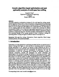
MR damper is a semi-active control device that uses controllable fluid [3]-[7]. This device is constructed by a hydraulic cylinder that contains MR fluid. MR fluids typically consist of micron-sized, magnetically polarizable particles dispersed in a carrier medium such as mineral or silicone oil. Commonly, the fluid is contains 20 to 40% by volume of relatively pure carbonyl iron with 3 to 5 microns in diameter. MR fluids could change their mechanical properties when they are exposed to a magnetic field. It is characterized by a great ability to vary, in a reversible way, from a free-flowing linear viscous liquid to a semi-solid one within milliseconds. Moreover, MR fluids can operate at temperatures from -40 to 150oC with only slight variations in the yield stress [5]. The structure of cylindrical type of MR damper and the behavior of MR fluid while encounters magnetic field is depicted in Fig. 1. Although, MR damper represents special features, highly nonlinear dynamics of the device hinders some unique characteristics of it and make the control process to have a precise and maybe complicated model. Many different models have been presented by a number of researchers in recent years that could be categorized in two groups: parametric and nonparametric. Basically, first one refers to models that represent the physical behavior of the device such as displacement, velocity, etc. while the second group refers to the black-box models that need just the experimental input-output data to simulate the device behavior. The most relevant parametric models to describe MR damper behavior are the Bingham model and its extended version proposed in [6] and [7] respectively; the hysteresis Bouc–Wen model [10] proposed in [5]; models, which include the Dahl friction model [11] proposed in [12]; the modified LuGre model [13]; the biviscous hysteretic model [14]; normalized form of Bouc-Wen model [15], which improved model performance by limited the hysteresis term in [-1,1], was employed in [16] and [17]. In non-parametric group some models such as [18], which used the combination of fuzzy logic and neural network; neural network models [19]; black box model [20]; models based on tracking curves by polynomials [21] and [22]; and some models, which employ genetic algorithm to optimize the parameters of parametric models such as [23] and [24], have been proposed. II. SIMULATION EXPERIMENTS AND COLLECTING DATA The experimental data for MR damper has employed to develop the fuzzy model, generated by using the base isolated benchmark program [25], which is used by the structural control community as a state-of-the-art model for numerical experience of seismic control attenuation. In fact, we use this

1035


numerical platform as a virtual laboratory test (Fig. 2). Therefore, four column data consisting of displacement, velocity, voltage, and force of MR damper are produced by employing seven predefined earthquake records of the benchmark problem and have been used as validation data.

(a)

(b)

Fig. 1 (a) Structure of MR damper [8]; (b) MR fluid behavior before and after applying magnetic field [9]

Fig. 2 Input-output data of the black box model of MR damper

It should be noted that the voltage refers to the corresponding fluctuating voltage of an earthquake, which is assessed by controller during full simulations. For training and checking data in the proposed approach, an Iranian earthquake record and a predefined earthquake record of the benchmark problem are employed. We use Nahavand record with peak ground acceleration (PGA) equal to 0.35, as an Iranian record, for training data, and Newhall earthquake record, as a predefined benchmark record, for checking data. Consequently, the model that is trained by Iranian earthquake would be validated by benchmark earthquakes records. The seven records were prepared to use in the benchmark program, but Nahvand record, first, should be pre-processed. Here, we used Seismosignal software, which is available in www.seismosoft.com, to apply base line correcting and filtering. Quadratic polynomial is used for base line correction. Butterworth filter and band-pass are used for filter type and filter configuration, respectively. [0.1, 25] is assumed as a desired interval for allowable frequencies. Nahavand earthquake record is shown in Fig. 3 before and after preparing. The corrected Nahavand earthquake record and Newhall earthquake record are shown in Fig. 4.

Fig. 3 (a) acceleration, (b) velocity, (c) displacement before and after correcting

Fig. 4 (a) Corrected Nahavand record in X direction, (b) predefined Newhall record of the benchmark program in Y direction

1036


The resulted Nahavand acceleration record in X direction is applied to benchmark program to generate training data as depicted in Fig. 5. Checking data, which is generated by applying Newhall acceleration record in Y direction, is shown in Fig. 6. It would be shown in the subsequent sections that how these data are employed to construct the proposed model.

Fig. 5 Training data: (a) displacement; (b) velocity; (c) controlled voltage; (d) generated force by applying Nahavand acceleration record in X direction to benchmark program

• GA’s flexibility facilitates both structure and parameter identification in complex models such as neural networks and fuzzy inference systems. The procedure of the algorithm is explained in the following. First, GA guesses randomly an initial population, which contains some chromosomes (depends on the specific problem). Each chromosome has some genes (equal to unknown parameters). Second, GA employs each chromosome in objective function, so the first generation would be evaluated. Finally, to obtain the better second generation, it uses selection, crossover, mutation, and elite operators. This process is repeated for all generation to optimize the objective function as well as possible. The final generation contains the best chromosomes, which contains the best genes (parameters values). It should be indicated that GA, in its traditional form, is based on the binary coding. In contrast, the new version employs real value of parameters. Generally, there is no regular rule to adjust the GA’s operators [29], and commonly they would be adjusted by trial and error. Reference [30], however, indicated that the operators are not independent to each other and they have some relationships. Therefore, in this paper, the algorithm is applied in way to avoid so many times of repetition in order to obtain the best performance of GA and also to apply in a way, which could be expanded to other optimization problems. The method of employing GA in the proposed model is explained in the next subsections. A. Population Size (N) Population size is the vital issue that influence significantly on the performance of the algorithm. It should cover a wide space of values. Reference [30] Proposed a simple but effective method for adjusting the population size, which has much better performance than other almost complicated approaches such as [31]-[34]. In this method, it is enough just to assess number of objective-function evaluation (FE):

Fig. 6 Checking data: (a) displacement; (b) velocity; (c) controlled voltage; (d) generated force by applying Newhall acceleration record in Y direction to benchmark program

FE 1 l . log(1 − ) = − M − log N N 12

III. GENETIC ALGORITHM Genetic algorithm (GA) [26] and [27], which was proposed for the first time by Holland from university of Michigan in 1975, is a free-derivative stochastic optimization method. This method, generally, is based on the natural process of human life, which selects parents (selection operator), produce a child who inherits his parents genes (crossover operator), sudden changing in genes (mutation operator), and transferring some best genes from parents with no change to a child (elite operator). The important attribute of GA is its independence to derivative information of the problem, which cause some deficiency in most optimizing work. The features of GA are as follows [28 p. 175]: • GA is parallel-search procedure that can be implemented on parallel processing machines for massively speeding up their operations. • GA is applicable to both continues and discrete combinatorial) optimization problems. • GA is stochastic and less likely to get trapped in local minima, which inevitably are present in any practical optimization application.

(1)

Where M is a constant, which appears during the process of obtaining the formula. In fact, it prevents the argument of logarithm to be zero. M=3 is suitable, and l is number of parameters. It is recommended that FE can be assumed, because of time and memory limitation, from the range [103,104]. B. Elite Operator This operator saves the best chromosome in any generation and transfers it with no changes to the next generation. In this paper, elite=2 is employed. The large number of this operator would cause the algorithm to be stagnated [30]. C. Selection Operator This operator decreases the deviation of objective function value by replacing the worse chromosome with better one. In fact, it looks for assessing parents. Reference [30] Chose Tournament for selection operator, which may weak GA performance. Here, the Uniform stochastic method is chosen.

1037


D.Crossover Operator This is the other vital operator of GA. After assessing the parents, this operator combines those chromosomes to produce a child chromosome. Here, scattered method is used, which has high performance. Meanwhile, crossover fraction = 0.8 is chosen. It means that crossover operator would influence on 80 percent of population, except elites, and remainder affected by mutation operator that is explained in next subsection E. Mutation Operator The most important attribute of this operator is covering the wide space of values by a sudden changing in some genes. Therefore, it prevents GA to be trapped in local minima. Reference [30] used the Uniform type of this operator that slows the performance of the algorithm. Here, Gaussian with scale=1 and shrink=1 is used F. The Criteria of Finishing In this paper, number of required generations to converge is chosen as the criteria to end GA. This is simply obtained by knowing the number of function evaluation (FE) and population size, which were assessed earlier:

g converge =

FE . N

(2)

G.Objective function Root mean squared error (RMSE) is contemplated as the objective function of GA:

RMSE =

1 n ∑ ( BM i − Modeli )2 , n i =1

(3)

where BMi is the ith data output, Modeli is the ith output of proposed model, and n is the size of a data. The proposed approach is explained in the next section to show how it would employ previous sections in an organized way. IV. MODELING METHODOLOGY In this paper the first order Takagi–Sugeno (TS) fuzzy model [35] and [36] is employed. To construct a TS fuzzy model of MR damper we should first select appropriate inputs. Based on numerical test that we have done on MR damper modeling, the inputs that has the significant influence on model performance are displacement, velocity, and voltage. This issue is also validated by relevant literatures such as [5], [17], and [18]. So we select these three inputs for our modeling purpose. Then the following cases should be done: • Selecting a data partitioning strategy to construct an initial structure of fuzzy model, • Applying a method to optimize the resulted structure. For the first one, we choose the well-known grid partitioning strategy. But the main concern is how many membership functions (MFs) for inputs have to be considered to make fuzzy IF–THEN rules. For the second one, it should be said that a fuzzy model just can approximate a plant behavior, which is the attribute of fuzzy models, but it cannot imitate the exact behavior of the plant. Combination of artificial neural network (ANN) and fuzzy logic system (FLS),

which is well-known as adaptive neuro-fuzzy inference system (ANFIS), have been used, which results trained fuzzy model [18]. The architecture, first employs least square estimator (LSE) in forward pass to estimate the consequent parameters of TS fuzzy model and next, it uses back-propagation learning, which consists of back-propagation method (to obtain gradient information of an objective function) and steepest descent method (to use the gradient information to update the parameters), to assess parameters of MFs in backward pass. However, since it is a gradient based method it might cause some deficiencies such as dependence on initial points and trapping in local minima; depending on the gradient descent (GD) methodologies and adjustment techniques. So it may not optimize the fuzzy model as well as possible. In this paper, we use GA as a derivative-free algorithm in our modeling approach. The proposed approach consists of two steps as follows: • Step 1. Estimating the number of MFs for each input individually by applying GA and LSE. • Step 2. Applying GA to assess the parameters of MFs (nonlinear part) and then estimating the consequent parameters (linear part) by LSE for each chromosome in generations of GA. In Step1, We introduce a fuzzy structure that has the training and checking data, which is explained before, with unknown number of MFs for each input to GA. Consequently, for each chromosome: first, GA estimates the number of MFs for each input based on grid partitioning strategy; second, the consequent parameters are estimated by LSE; finally, by contemplating the training and checking data error simultaneously, the algorithm would assess the optimize number of MFs for each input. The only constraint in this step is the maximum number of MFs for inputs and also the maximum number of rules (because the same number of rules could occur with different arrangement of MFs for each input). In Step 2, the resulted structure would be introduced to GA, in order to find the optimized parameters of MFs while the consequent parameters are estimated by LSE. In fact, if we want to compare the proposed method by ANFIS in this step, the back-propagation learning (derivative based) stage is replaced by GA (derivative-free) just with one forward pass. Therefore, the randomness and stochastic nature of GA leads the optimization process to a global minimum. V. MODEL DEVELOPMENT In this section we employ the proposed approach to imitate the behavior of MR damper. The training and checking data consists of 9470 and 6000 data pairs as were shown in Fig. 5 and Fig. 6, respectively. In step 1, MFs=[6 6 6] and rules = 24 (because of time limitation) are assumed as the maximum number of MFs for each input and the maximum number of rules, respectively. We use generalization bell function (g-bell) as type of MFs. Due to the a few numbers of parameters, FE=103 is assumed, so N=10 and gconverge=100 are obtained from (1) and (2),

1038


respectively. MFs=[2 6 2] is obtained after 5 runs of GA, which belongs to displacement, velocity, and voltage data, respectively.In step 2, the resulted structure is introduced to the combination of GA and LSE, as explained before. Consequently, 30 optimized nonlinear parameters and 96 optimized linear parameters would be obtained. Meanwhile, because of more unknown parameters in this step, GA is calibrated as FE=104, N=40 and gconverge=250. Fig. 7 and Fig. 8 show the initial and final MFs.

Fig. 7 Initial MFs on displacement, velocity and voltage, which are located evenly in their specific intervals

Fig. 8 Final MFs on displacement, velocity and voltage, which are estimated by GA in step 2

More number of MFs on velocity, which is obtained automatically in Step 1 of the proposed approach, shows its significant role in the behavior of MR damper. Fuzzy logic, which is expressed the approximate human knowledge, basically emerged to approximate a plant behavior and simultaneously to be interpretable. But since the aim is imitating the exact behavior of a plant, using an optimization method is inevitable. Consequently, as long as an optimization method is used the model accuracy would increase; however, simultaneously the model capability to be interpretable may decrease. The case that could occur, for example, in ANFIS performance as depicted in [28 p. 341].

Fig. 9 Comparison the proposed model predicted force (F) with the target force (FBM); Force vs. (a) Time, (b) Displacement, (c) Velocity, (d) Voltage under Nahavand excitation (training data)

This issue could be seen in velocity MFs, as it is shown in Fig. 8, which are overlapped and cannot be interpreted. Moreover, one interesting point to be said, is up-side down MFs on velocity, which is due to the negative amount of parameter b in g-bell function (gbellmf(x,[a b c])); the case that is rare in ANFIS method.

1039


training data was its wide range of input-output data, which it could cover the input-output data range of all seven predefined benchmark records. This is a principle issue when we want to select a training data and it directly influence on model performance. In this paper we also modeled MR damper based on ANFIS method, which is one of the well-known methods in soft computing framework, in order to compare it with the proposed model. The RMSE (3) for training and checking data are listed in Table I, where ANFIS was run for different epoch number. TABLE I THE RMSE VALUES FOR BOTH ANFIS AND PROPOSED METHOD FOR TRAINING AND CHECKING DATA

Method

MFs

Epoch

RMSEtraining

RMSEchecking

ANFIS ANFIS Proposed approach

[2 6 2] [2 6 2]

100 1000

73.05 63.09

115.11 101.23

[2 6 2]

1

43.67

52.12

Although the training error in proposed model is less than ANFIS method, the large checking data error in ANFIS is significant. In contrast, the checking data error in the proposed approach is close to training data error. This would occur because for both steps in GA part of proposed approach the training and checking data errors are included in the objective function; thus, it causes decrease in both errors simultaneously and approximately equally. This is a specific attribute of the proposed approach. Moreover, as it can be seen from Table I, 10 times increasing the number of epoch only results in small changes in the errors. The RMSE for the all seven earthquake records are brought in Table II, where the excellent performance of the proposed approach is seen. TABLE II RMSE VALUES FOR THE PROPOSED MODEL AND ANFIS (EPOCH=1000). EACH CELL CONTAINED X AND Y DIRECTION OF EARTHQUAKE RECORDS INFORMATION AT THE TOP AND BOTTOM, RESPECTIVELY Method ANFIS Proposed approach

Fig. 10 Comparison the proposed model predicted force (F) with the target force (FBM); Force vs. (a) Time, (b) Displacement, (c) Velocity, (d) Voltage under Newhall excitation (checking data)

Comparing the force, which is predicted by the proposed approach (F), with the target force (FBM), from the benchmark program, are depicted in Fig. 9 and Fig. 10 for the training and checking data, respectively. Fig. 9 and Fig. 10 show the excellent performance of the proposed approach not only for training data but also for checking data. It should be said the reason that we selected Nahavand earthquake record as a

Newhall

Sylmar

123.37 101.23 63.22 52.12

101.85 114.57 52.58 58.24

El Centro 121.85 166.66 62.24 111.80

Rinaldi

Kobe

Jiji

Erzinkan

99.47 121.95 57.05 63.22

130.17 91.60 119.50 65.38

92.08 122.03 65.29 51.46

86.60 99.87 56.60 52.21

In the relevant literature, comparing nonparametric models with parametric one rarely have been done. Although the parametric models have some deficiencies, because of employing strict and precise mathematical differential equation to describe the nonlinear and inherent dynamics of MR damper, they have a high accuracy and are superior to nonparametric models. [16] and [17] are the two best parametric models for describing the behavior of MR damper, which they used normalized Bouc-Wen term for hysteresis phenomenon. In order to compare, we use the same performance index (PI) as [17] did. It is the 1-norm error (ε) which is defined as follows: Tr F −F 1 , (4) f 1 = ∫ f (t ) dt ε= d 0 Fd 1 Where FBM is the target force (benchmark building platform

1040


output) and F is the resulting force of the proposed approach. The results are listed in Table III. TABLE III

ε VALUES IN TERMS OF % FOR THE PROPOSED MODEL, ANFIS (EPOCH=1000), AND TWO PARAMETRIC MODELS. EACH CELL CONTAINED X AND Y DIRECTION OF EARTHQUAKE RECORDS INFORMATION AT THE TOP AND BOTTOM, RESPECTIVELY. (THE TWO FIRST ROWS ARE FROM [17]) Method

Newhall

Sylmar

Parametric 1

6.47 3.84

5.67 8.44

El Centro 7.78 7.90

Rinald i 7.12 5.67

Parametric 2

16.15 15.83

18.06 24.14

22.89 19.68

17.55 18.48

ANFIS

9.96 8.80

7.50 6.36

12.21 14.75

6.83 5.76

Kobe

Jiji

6.52 7.85 18.2 2 24.7 2 9.90 20.2 9

3.61 4.02 14.1 6 20.0 9 9.25 8.94

Erzinka n 4.88 5.35 14.19 18.80 5.50 4.58

Table III shows that the proposed model has better performances even in comparison with parametric models.Furthermore, it should be noted that, although the Parametric 1 method has a good performance, it could not be inversed. In contrast, the proposed model easily can be inversed just by interchanging the force and voltage location in the data. The model capability for being inversed is a vital issue when we want to apply the model to a control process where an appropriate instant voltage signal should be sent to MR dampers during an earthquake. Consequently, the proposed approach, which could be categorized in soft computing techniques, can have promising role in modeling and control process. REFERENCES [1] [2] [3]

[4]

[5]

[6] [7]

[8]

[9]

[10] [11] [12] [13] [14]

Soong T T and Dargush G F 1997 Passive Energy Dissipation Systems in Structural Engineering (UK: Wiley). Soong T T and Spencer B F Jr 2002 Supplemental energy dissipation: state-of-the-art and state-of-the-practice Eng.Struct. 24 243259. Choi S B, Lee S K and Park Y P 2001 A hysteresis model for fielddependent damping force of a magnetorheological damper J. Sound Vib. 245 375–83. Jolly M R, Bender J W and Carlson J D 1999 Properties and applications of commercial magnetorheological fluids J. Int. Mater. Syst. Struct. 101 5–13. Spencer B F Jr, Dyke S J, Sain M K and Carlson J D 1997 Phenomenological model for a magnetorheological damper ASCE J.Eng. Mech. 123 230–52. Stanway R, Sproston J L and Stevens N G 1987 Non-linear modelling of an electro-rheological vibration damper J. Electrostat. 20 167–84. Gamota D R and Filisko F E 1991 Dynamic mechanical studies of electrorheological materials: moderate frequencies J. Rheol. 35 399– 425. G. Yang, Large-scale magnetorheological fluid damper for vibration mitigation: Modeling, testing and control, Ph.D dissertation,University of Notre Dame (2001). M. Kciuk and R. Turczyn, Properties and application of magnetorheological fluids, Journal of Achievement in Material and Manufacturing Engineering 18 (2006), no. 1-2, 127–130. Wen Y K 1976 Method of random vibration of hysteretic systems ASCE J. Eng. Mech. 102 249–63. Dahl P R 1968 A solid friction model Technical Report TOR-158(310718) (El-Segundo, CA: The Aerospace Corporation) Ikhouane F and Dyke S J 2007 Modeling and identification of a shear mode magnetorheological damper Smart Mater. Struct.16 605–16. Jimenez R and Alvarez-Icaza L 2004 LuGre friction model for a magnetorheological damper Struct. Cont. Health Monit.20 91–116. Guo S, Yang S and Pan C 2006 Dynamic modeling of magnetorheological damper behaviors J. Int. Mater. Syst.Struct. 17 3– 14.

[15] Ikhouane F, Rodellar J. Systems with hysteresis: analysis, identification and control using the Bouc–Wen model. John Wiley and Sons Inc.; 2007. [16] Rodriguez A, Ikhouane F, Rodellar J, Luo N. Modeling and identification of a small-scale magnetorheological damper. J Intell Mater Syst Struct 2009;20(7):825–35. [17] Bahar A, Pozo F, Acho L, Rodellar J, Barbat A. Parameter identification of large scale magnetorheological dampers in a benchmark building. Computers and Structures 2010;88:198-206. [18] Schurter KC, Roschke PN. Fuzzy modelling of a magnetorheological damper using ANFIS. In: Proc. 9th IEEE intl conf on fuzzy systems. 2000.p. 122-7. [19] Wang DH, Liao WH. Modeling and control of magnetorheological fluid dampers using neural networks. Smart Materials and Structures 2005;14(1):111-26. [20] Jin G, Sian MK, Spencer Jr BF. Nonlinear blackbox modeling of MRdampers for civil structural control. IEEE Transactions on Control Systems Technology 005;13(3):345-55. [21] Choi SB, Lee SK. A hysteresis model for the field-dependent damping force of a magnetorheological damper. Journal of Sound and Vibration 2001;245(2):375-83. [22] Ma XQ,Wang ER, Rakheja S, Su CY. Modeling hysteretic characteristics of MR-fluid damper and model validation. In: Proc. 41st IEEE conf. On decision and control. 2002. p. 1675-80. [23] Giuclea M, Sireteanu T, Stanciou D, Stammers CW. Model parameter identification of vehicle vibration control with magnetorheologicaldampers using computational intelligent methods. Proceedings of the Institution of Mechanical Engineers. Part I: Journal of Systems and Control Engineering 2004;218:569-81. [24] N.M. Kwok_, Q.P. Ha, M.T. Nguyen, J. Li, B. Samali Bouc-Wen model parameter identification for a MR fluid damper using computationally efficient GA. 0019-0578/$ - see front matterc 2007, ISA. Published by Elsevier Ltd. p.167-179. [25] Narasimhan S, Nagarajaiah S, Johnson EA, Gavin HP. Smart baseisolated benchmark building. Part I: problem definition. Struct Control Health Monitor 2006;13(2-3):573-88. [26] J.H. Holland. Adaptation in natural and artificial systems. University of Michigan Press,Michigan ,1975. [27] Goldberg DE. Genetic algorithms in search, optimization and machine learning. Reading (MA): Addison-Wesley; 1989. [28] Jang JR, Sun CT, Mizutani E. Neuro-fuzzy and soft computing. Prentice-Hall International Inc. 1997. [29] Eiben AE, Hinterding R, Michalewicz Z. Parameter control in evolutionary. algorithms. IEEE Transactions on Evolutionary Computation 1999;3(2):124-41. [30] Matthew S. Gibbs,1, Graeme C. Dandy, Holger R. Maier. A genetic algorithm calibration method based on convergence due to genetic drift.0020-0255/$ - see front matter _ 2008 Elsevier Inc. p.2857-2869. [31] J. Arabas, Z. Michalewicz, J.J. Mulawka, GAVaPS - a genetic algorithm with varying population size., in: International Conference on Evolutionary Computation, 1994, pp. 73-78. [32] T. Bäck, A.E. Eiben, N. van der Vaart, An empirical study on GAs ‘‘without parameters”, in: M. Schoenauer, K. Deb, G. Rudolph, X. Yao, E. Lutton,J.J. Merelo, H.-P. Schwefel (Eds.), Parallel Problem Solving from Nature—PPSN VI of Lecture Notes in Computer Science, vol. 1917, Springer-Verlag,Paris, France, 2000, pp. 315-324. [33] A.E. Eiben, E. Marchiori, V.A. Valko, Evolutionary algorithms with onthe-fly population size adjustment, in: X. Yao, E. Burke, J. Lozano,J. Smith, J. Merelo-Guervós, J. Bullinaria, J. Rowe, P. Tino, A. Kabán, H.P. Schwefel (Eds.), Parallel Problem Solving from Nature—PPSN VIII of Lecture Notes in Computer Science, vol. 3242, Springer, 2004, pp. 41-50. [34] K. Srinivasa, K. Venugopal, L. Patnaik, A self-adaptive migration model genetic algorithm for data mining applications, Information Sciences 177 (20) (2007) 4295-4313.. [35] T. Takagi and M. Sugeno, “Fuzzy identification of systems and its applications to modeling and control,” IEEE Trans. Syst., Man, Cybern., vol. SMC-15, no. 1, pp. 116-132, Feb. 1985. [36] M. Sugeno and G. T. Kang. Structure identification of fuzzy model. Fuzzy Sets and Systems, 28:15-33, 1988.

1041