An Optimization Framework for Map-Reduce Queries - Semantic Scholar

An Optimization Framework for Map-Reduce Queries Leonidas Fegaras,

Chengkai Li,

Upa Gupta

University of Texas at Arlington, CSE Arlington, TX 76019 {fegaras,cli,upa.gupta}@uta.edu

ABSTRACT We present an effective optimization framework for general SQLlike map-reduce queries, which is based on a novel query algebra and uses a small number of higher-order physical operators that are directly implementable on existing map-reduce systems, such as Hadoop. Although our framework is applicable to any SQL-like map-reduce query language, we focus on a powerful query language, called MRQL. Current map-reduce query languages, such as HiveQL and PigLatin, enable users to plug-in custom map-reduce scripts into queries for those jobs that cannot be declaratively coded in the query language, which may result to suboptimal, error-prone, and hard-to-maintain code. In contrast to these languages, MRQL is expressive enough to capture most of these computations in declarative form and at the same time is amenable to optimization. We describe an optimization framework that maps the algebraic forms derived from the MRQL queries to efficient workflows of mapreduce operations that consist of our physical plan operators. We also describe many algebraic optimizations, such as fusing cascading map-reduce jobs into one job and synthesizing a combine function from the reduce function of a map-reduce job. Finally, we report on a prototype system implementation and we show some performance results of evaluating MRQL queries on a small cluster of computers.

1.

INTRODUCTION

The map-reduce (MR) programming model [10] is a popular framework for cloud computing that enables large-scale data analysis on the cloud. It facilitates the parallel execution of ad-hoc, longrunning, large-scale data analysis tasks on a shared-nothing cluster of commodity computers connected through a high-speed network. Although the MR framework is used extensively by companies on a very large scale, it is still a controversial topic within the database community, especially when compared to parallel databases [24]. While current databases require the programmer to first model and load the data before processing, the MR model is better suited to one-time ad-hoc queries over write-once raw data (in situ data). In addition, MR platforms offer better fault tolerance and the abil-

ity to operate in heterogeneous environments, which is crucial for cloud computing. Finally, while data indexing is very important in attaining high performance in relational databases, it may not be applicable to an MR environment due to the transience of data. Many data analysis tasks need to process most of the data, in which case indexes are not very useful, or, when parts of the data are needed, the amortized cost of index creation/population may exceed the cost benefit of using the index. Nevertheless, there are some recent systems that try to bridge the gap between the MR and RDB frameworks by providing some higher-level declarative language that makes MR programming easier (such as HiveQL [25] and PigLatin [22]) or by extending the MR framework with indexing and optimizations (such as HadoopDB [1] and Manimal [18]). The basic idea behind an MR framework is simple. For each MR job, one needs to provide a map and a reduce task. The map task specifies how to process a single key/value pair to generate a set of intermediate key/value pairs while the reduce task specifies how to merge all intermediate values associated with the same intermediate key. MR tasks can be arbitrary computations coded in a general-purpose programming language. The MR framework uses the map task to process all input key/value pairs in parallel by distributing the data among a number of nodes in a cluster (the map workers), which execute the map task in parallel without communicating with each other. Then, the map results are repartitioned across a number of nodes (the reduce workers) so that values associated with the same key are grouped and processed by the same node. Finally, each reduce worker applies the reduce task to every group in its assigned partition. MR engines use a distributed file system (DFS), spread across the worker nodes, to store and replicate data. The entire MR computation is controlled by a designated coordinator (the job tracker) and each node uses a task tracker to control its own tasks. It is well-known that standard SQL queries (simple queries that use joins, selections, projections, group-by, having, and order-by) can be directly coded into simple MR workflows [10], although the choices for join implementations in MR can be quite limited compared to relational databases. For example, the SQL query: select v.A, sum(v.B) from R as v group by v.A

can be coded in MR using the following Java pseudo-code:

Permission to make digital or hard copies of all or part of this work for personal or classroom use is granted without fee provided that copies are not made or distributed for profit or commercial advantage and that copies bear this notice and the full citation on the first page. To copy otherwise, to republish, to post on servers or to redistribute to lists, requires prior specific permission and/or a fee. EDBT 2012, March 26–30, 2012, Berlin, Germany. Copyright 2012 ACM 978-1-4503-0790-1/12/03 ...$10.00

class Mapper method map ( key, v ) emit(v.A,v); class Reducer method reduce ( key, values ) int c = 0; for each v ∈ values do c += v.B; emit(key,c); where the emit method appends key/value pairs to the output stream.

That is, for each tuple v from R, the mapper emits the pair (v.A,v), so that these pairs are grouped by the key v.A and each group is passed to the reducer as a collection of values associated with the same key. Then, for each group, the reducer sums up all the v.B values and emits the final result. Although standard SQL can be coded in MR, not all MR jobs can be coded in SQL. In fact, MR programs over a relation R are computationally complete, since the reducer can be a computationally complete function and we can use a mapper that emits the same key for all tuples in R, sending all R tuples into the same group for reduction. Even though, in principle, the MR model is very simple to understand, it is hard to develop, optimize, and maintain non-trivial MR applications coded in a general-purpose programming language. In addition, there are many configuration parameters to adjust for better performance that overwhelm non-expert users. As is evident from the success of the relational database technology, program optimization would be more effective if data processing programs were written in a declarative query language that hides the implementation details and is amenable to optimization. Existing MR query languages, such as HiveQL [25] and PigLatin [22], provide a limited syntax for operating on data collections, in the form of relational joins and group-bys. Because of these limitations, these languages enable users to plug-in custom MR scripts into their queries for those jobs that cannot be declaratively coded in their query language. This nullifies the benefits of using a declarative query language and may result to suboptimal, error-prone, and hard-tomaintain code. To appreciate what is required to capture all MR computations declaratively in SQL-like syntax, consider a general MR job over a single relation R that groups the tuples of R using the map function m and then applies the reduce function r to each group. It can be represented by the following SQL-like code: select k, r (values) from R as v group by k: m(v)

This query groups the tuples v of R using the group-by key k = m(v). After the group-by, the variable values will contain a group, that is, all tuples associated with the same m(v) key. This query, of course, cannot be directly coded in standard SQL but describes what exactly needs to be achieved to reach MR completeness. SQL does not allow m and r to be nested queries and does not support access to the entire group, values, other than performing simple aggregations over the group elements. Consequently, nested queries are essential for achieving MR completeness in an MR query language. They are also very important as they appear in many common data analysis queries. Consider, for example, the following SQL-like query that calculates one step of the k-means clustering algorithm (Lloyd’s algorithm), by deriving k new centroids from the old: select avg(s.X) as X, avg(s.Y) as Y, avg(s.Z) as Z from Points as s group by (select ∗ from Centroids as c order by distance(c,s))[0]

where Points is the input data set (3D points), Centroids is the current set of centroids (k cluster centers), and distance calculates the distance between two points. The inner query assigns the closest centroid to a point s (where [0] returns the first tuple of an ordered list). This query clusters the data points by their closest centroid, and, for each cluster, a new centroid is calculated from the mean values of its points. Most SQL implementations do not allow subqueries in group-by nor they allow arbitrary operations over groups and, therefore, have insufficient expressive power to achieve MR completeness. There are other query languages though, such as ODMG OQL, that allow both. Finally, the query language must support hierarchical data and nested collections uniformly, allow-

ing us to query JSON and XML data, such as the content dumps in XML format provided by Wikipedia. This capability is far more important for MR queries than for SQL, because, although data can be normalized before they are stored in a relational database, raw data must be processed as is, even if they are nested. Finally, the query language must support recursion or transitive closure declaratively, to capture graph algorithms, such as PageRank. Our framework uses a novel query language for map-reduce computations, called MRQL (the Map-Reduce Query Language) [13], that is more powerful than existing query languages, such as Hive and PigLatin, since it can operate on more complex data, such as nested collections and trees, and it supports more powerful query constructs, thus eliminating the need for using explicit MR procedural code. It is powerful enough to capture most commonly used MR computations declaratively, is easy to learn, has uniform syntax, is extensible, has simple semantics, and can be compiled to efficient MR programs. It is important to note that the main contribution of this paper is not in the language itself. In fact, we could have used some other suitable language that satisfies the requirements listed above, such as OQL or XQuery. Instead, the contribution of our work is in the design and implementation of an effective optimization framework for MR queries. We believe that our optimizations can apply to other suitable MR query languages too. When building an MR query optimizer, we can certainly leverage on the existing relational query optimization technology, especially on the techniques used in distributed databases. There are some important differences though that make MR query optimization challenging. First, the MR physical operators are different from those used by RDBMSs since they have to be expressed as MR jobs. Second, MRQL queries are far harder to optimize than SQL queries, since they allow arbitrary query nesting and nested collections. Third, there are some specific optimizations that apply to MR jobs only, such as synthesizing the combine function from a reduce function. A combine function is an optional MR task that applies to the data generated at each map task to partially reduce the data at the map-side before they are shuffled and shipped to the reducers. The combine step is very effective if the reducer performs aggregations only, because it lessens the amount of shipped data. The first challenge faced when designing a query algebra for MR queries is evaluating nested queries efficiently. Nested queries are essential for achieving MR completeness in an MR query language and they deserve special optimization techniques. We would like to generalize relational joins to cope with arbitrary nested queries in a way that is more suitable to an MR framework. Consider, for example, the nested SQL query: select ∗ from X as x where x.D > (select sum(y.C) from Y as y where x.A=y.B)

A typical method for evaluating this query in a RDBMS is to first group Y by y.B, yielding pairs of y.B and sum(y.C), and then to join the result with X on y.B=x.A using a right-outer join, removing all those matches whose x.D is below the sum. Unfortunately, this method can be suboptimal in an MR environment because it requires two MR jobs, one for the group-by and one for the join. Instead, this query can also be evaluated with one reduce-side join [27], which requires only one MR job. Furthermore, although the grouping and aggregation are done during the reduce phase of the reduceside join, one can use in-mapper combining [27] to partially aggregate data before reduction. This reduce-side join plan is in many cases more efficient than the RDBMS group-by/join plan and a good optimizer should be able to select the best based on cost. The fundamental reason that makes it hard for a traditional RDBMS optimizer to recognize opportunities for fusing a group-by with a join into a reduce-side join is that relational joins were designed to

produce flat data (by concatenating the joined tuples), since this is the only kind of data supported by the relational model. This requires that a group-by must always be combined with aggregations to produce flat data. But there is no reason for doing so for a data model that supports nested collections. In fact, instead of concatenating the x and y tuples, we can nest them in a way that reflects the query nesting. For our example, the join between X and Y can deliver pairs of (x,ys), such that ys is the collection of all y in Y that are joined with an x from X. That way, the predicate can be executed directly in memory using x.D > (select sum(y.C) from ys as y), without using an explicit group-by. Our work generalizes this idea to handle arbitrary nested queries, at any place, number, and nesting level (described in Section 6). For an MR query language to be useful, in addition to its expressive power, it must run efficiently on a given MR platform and it should consume resources at a rate comparable to procedural code written by experts. Failure to do so would divert programmers from using this query language, who will choose to sacrifice declarativeness for efficiency. Consider for example the popular PageRank algorithm that measures the relative importance of nodes in a graph. Efficient implementations of PageRank on an MR platform have been extensively investigated in the literature [20]. These methods use various tricks to improve performance, such as propagating the entire graph at each iteration step to avoid recovering the graph using a join. In general, these methods require a single MR job at each iteration step. PageRank can be expressed in SQL as follows. The graph is represented as a set of links, where each link has a source and a destination dest, but also repeats some information about the source: the total number of its outgoing links count and its PageRank rank (which is improved at each iteration). A simplified version of the PageRank algorithm can be expressed as a repetition of the following SQL query that derives a new set of edges from the old set, changing only their rank (the complete query expressed in MRQL is given in Figure 4 in Section 7): select m.source, m.dest, m.count, c.rank from (select n.dest, sum(n.rank/n.count) as rank from Graph as n group by n.dest) as c, Graph as m where m.source = c.dest

That is, the inner query reverses the graph by grouping the links by their link destination and it equally distributes the rank of the link sources to their destination. The outer select-query recovers the graph by joining the new rank contributions with the original graph so that it can be used in the next iteration step. This query, if evaluated naively, requires two MR jobs: one MR job to group the nodes by their destination (inner query), and one MR job to join the rank contributions with the nodes (outer query). Our system translates this query to one MR job by using the following two algebraic laws (these rules are described in detail in Section 6.4): 1. A group-by before a join can be fused with the join if the group-by attribute is the same as the corresponding join attribute. The resulting reduce-side join nests the data during the join, thus incorporating the group-by effects. 2. A reduce-side self-join (which joins a dataset with itself) can be simplified to an MR job that traverses the dataset once. In essence, the map function of this MR job sends each input element to the reducers twice under different keys: under the left and under the right join keys. That is, the group-by operation in this query can be fused with the join, based on the first rule, deriving a self-join, which, in turn,

can be simplified to a single MR job, based on the second rule. These algebraic optimizations capture the essence of the ad-hoc techniques used by programmers to improve their PageRank MR jobs. These and other algebraic laws can only be expressed and validated if MR jobs, reduce-side joins, and other MR operations, are expressed in a suitable formal algebra with precise semantics. In summary, the key contribution of this work is in the design and implementation of an effective optimization framework for MR query languages that has the following characteristics: • It provides a small but powerful set of physical plan operators that are directly implementable on existing map-reduce systems, such as Hadoop. It also gives the precise semantics of these physical operators and their implementation in Hadoop. • It defines an MR algebra with precise semantics, which consists of a small number of higher-order operators that are powerful enough to capture all MRQL language constructs. The most important algebraic operator is the join operation that generalizes the relational join by incorporating data grouping into the join. This join can nest the join results in such a way that nested queries can be evaluated without the need of additional group-by operations. • It uses novel optimization techniques to translate MRQL queries to algebraic forms and to map these algebraic forms to efficient workflows of physical plan operations. It provides many algebraic optimizations, such as fusing cascading MR jobs into a single job and synthesizing a combine function from the reduce function of an MR job. • It uses a cost-based heuristic optimizer to derive an efficient physical plan from a query graph. Currently, our cost model is incomplete as it takes into account the input dataset sizes and the available resources but, due to lack of statistics, it assumes constant predicate selectivities. • Finally, it is implemented on top of Hadoop, without requiring any change to the system. It can process complex MRQL queries over XML, JSON, binary, and record-oriented text documents. The rest of this paper is organized as follows. Section 2 compares our approach with related work. Section 3 describes the syntax of MRQL and gives some examples of queries. Section 4 describes our physical plan operators and Section 5 describes our algebra. Section 6 describes our methods for translating MRQL to physical plans and for optimizing these plans. Finally, Section 7 reports on a prototype implementation of MRQL using Hadoop and evaluates the performance of PageRank queries on a small cluster.

2. RELATED WORK The map-reduce (MR) model was first introduced by Google in 2004 [10]. Several large organizations have implemented this model, including Apache Hadoop [27] and Pig [22], Apache/Facebook Hive [25], Google Sawzall [23], and Microsoft Dryad [16]. The most popular MR implementation is Hadoop [15], an opensource project developed by Apache, which is used today by Yahoo! and many other companies to perform data analysis. There are also a number of higher-level languages that make MR programming easier, such as HiveQL [25], PigLatin [22], SCOPE [8], and Dryad/Linq [17]. There are several join algorithms for the MR framework, such as reduce- and map-side joins [20, 27].

Hive [25, 26] is an open-source project by Facebook that provides a logical RDBMS environment on top of the MR engine, well-suited for data warehousing. Using its high-level query language, HiveQL, users can write declarative queries, which are optimized and translated into MR jobs that are executed using Hadoop. HiveQL does not handle nested collections uniformly: it uses SQLlike syntax for querying data sets but uses vector indexing for nested collections. Unlike MRQL, HiveQL has many limitations (it is a small subset of SQL). It does not allow query nesting in predicates and select expressions, but allows a table reference in the from-part of a query to be the result of a select-query. Because of these limitations, HiveQL enables users to plug-in custom MR scripts into queries. Although Hive uses simple rule-based optimizations to translate queries, it has yet to provide a comprehensive framework for cost-based optimizations. Yahoo!’s Pig [14] resembles Hive as it provides a user-friendly query-like language, called PigLatin [22], on top of MR, which allows explicit filtering, map, join, and group-by operations. Like Hive, PigLatin performs very few optimizations based on simple rule transformations. PACT/Nephele [3] is an MR programming framework based on workflows, where each workflow component can be a map or reduce. These workflows are converted to logical execution plans for Nephele, a general distributed program execution engine. Even though PACT/Nephele workflow programs are very flexible and are not limited to rigid map/reduce pairs, they are hard to program, since programmers have to construct low-level workflows. SCOPE [8], an SQL-like scripting language for large-scale analysis, does not support sub-queries but provides syntax to simulate sub-queries using outer-joins. Like Hive, because of its limitations, SCOPE provides syntax for user-defined process/reduce/combine operations to capture explicit MR computations. HadoopDB [1] adopts a hybrid scheme between MR and parallel databases to gain the benefit of both systems. Although, HadoopDB uses Hive as the user interface layer, instead of storing table tuples in DFS, it stores them in independent DBMSs in each physical node in the cluster. That way, it increases the speed of overall processing as it pushes many database operations into the DBMS directly, and, on the other hand, it inherits the benefits of high scalability and high fault-tolerance from the MR framework. Hadoop++ [11] decomposes each MR computation into an execution plan and then transforms it to take advantage of possible indexes attached to data splits. It does not provide a framework for recognizing joins and filtering in general MR programs, to take advantage of the indexes. Manimal [7, 18] analyzes the MR code to find opportunities for using B+-tree indexes, projections, and data compression. Finally, the Asterix project [4] shares some of our goals but it has a broader scope and has far more ambitious plans. It proposes a scalable platform to store, manage, and analyze large volumes of semistructured data. Unlike our approach, instead of using an existing distributed file system combined with a parallel processing framework, such as Hadoop, Asterix uses its own distributed data store, called Hyracks [5]. Hyracks was designed from the groundup to directly support the parallel algorithms needed for evaluating complex declarative queries and at the same time to offer scalability, reliability, and availability. There are plans to develop a costbased optimizer for the Asterix query language, which is influenced by XQuery, but, as far as we know, there is no comprehensive query optimization framework developed yet.

3.

THE MRQL MODEL AND LANGUAGE

In this section, we briefly overview the MRQL data model and query language. Due to lack of space, we left this description incomplete since the focus of this paper is not on the language it-

self, but on a comprehensive query optimization framework that can optimize map-reduce query languages like this. The complete description of MRQL can be found at the project web page [21]. We assume that the input data sources are raw text or binary files. The MRQL expression that makes a directory of raw files accessible to a query is: source( parser, uri, ... )

where uri is the URI of the directory that contains the files, parser is the name of a function that parses enough bytes from a file to construct a single fragment, and ‘...’ are parser-specific parameters. The parser must be stateful so that consecutive calls to the parser return consecutive fragments from the files. We have experimented with three different parsers: an XML parser, a JSON parser, and a line-based parser that generates one relational record from each input line containing values separated by a user-defined delimiter. For brevity, from now on, we will use names for data sources, instead of source calls. The MRQL query syntax has been influenced by ODMG OQL, the OODB query language developed in the 90’s, while its semantics has been inspired by the work in the functional programming community on list comprehensions with group-bys and orderbys [19]. In its simplest form, the select-query syntax in MRQL is as follows: select [ distinct ] e from p1 in e1 , . . . , pn in en [ where ec ] [ group by p′ : e′ [ having eh ] ] [ order by eo [ limit n ] ]

where all these e’s are arbitrary MRQL expressions, which may contain other nested select-queries. MRQL handles a number of collection types, such as lists (sequences), bags (multisets), and key/value maps. The difference between a list and a bag is that a list supports order-based operations, such as indexing. An MRQL query works on collections of values, which are treated as bags by the query, and returns a new collection of values. If it as an order-by query, the result is a list, otherwise, it is a bag. Treating collections as bags is crucial to our framework because it allows the queries to be compiled to MR programs, which need to shuffle and sort the data before reduction, and enables the use of joins for query evaluation. The from part of an MRQL syntax contains query bindings of the form ‘p in e’, where p is a pattern and e is an MRQL expression that returns a collection. The pattern p matches each element in the collection e, binding its pattern variables to the corresponding values in the element. In other words, this query binding specifies an iteration over the collection e, one element at a time, causing the pattern p to be matched with the current collection element. In general, a pattern can be a pattern variable that matches any data, a tuple (p1 , . . . , pn ) or a record that contains patterns pi . For example, the following query: select (n,cn) from < name: n, children: cs > in Employees, < name: cn > in cs

iterates over Employees, and for each employee record, it matches the record with the pattern , which binds the variables n and cs to the record components name and children, respectively, and ignores the rest. Without patterns, this query is equivalent to: select (e.name,c.name) from e in Employees, c in e.children

This is a dependent join because the domain of the query variable c depends on e.

The group-by syntax of an MRQL query takes the form group by p′ : e′ to partition the query results into groups so that the members of each group have the same value e′ . The pattern p′ is bound to the group-by value, which is common across each group. As a result, the group-by operation lifts all non-group-by pattern variables (defined in the from-part of the query) from some type T to a bag of T , indicating that each such variable must contain multiple values, one for each member of the group. For example, the query select ( d, c, sum(s) ) from in Employees group by (d,c): ( dn, s>=100000 )

groups Employees by dno and by whether their salary is greater than 100K. The variables d and c in the query header are directly accessible since they are group-by variables. The variable s in sum(s), on the other hand, is lifted to a bag of integers, which contains the salaries of employees in a group. In contrast to SQL, the function sum does not require a special semantics; it is simply a user-defined function from a bag of integers to an integer. Finally, the ‘order by’ syntax orders the result of a query (after the optional group-by) by the e0 values. (There is a default total order ≤ defined for all data types, including tuples and bags.) Graph algorithms, such as PageRank, require repetitive applications of MR jobs, that can be expressed as transitive closures or recursion. In MRQL, a repetition takes the form: repeat v = e step body [ limit n ]

where v is the repetition variable. The type of e must be a bag(T ), for some type T , and the type of body must be bag( (T ,bool) ). This expression first binds v to the value of e and then it evaluates the body repeatedly and assigns a new value to v from the previous value, which is derived from the first components of the pairs returned by body. It stops if either the number of repetitions becomes n or when all the booleans returned by body are false. Figure 4 in Section 7 shows a PageRank query that uses repetition.

4.

THE MRQL PHYSICAL OPERATORS

The main goal of this paper is to translate MRQL queries to efficient workflows of MR jobs. In addition to the generic MR operation, which can be parameterized with a map and a reduce function, we would like to design a number of specialized computations that can perform some operations needed by MRQL queries, such as equi-joins. That is, we would like to design a number of physical evaluation operators that explicitly capture the MRQL functionality and are directly implementable on any existing MR environment, such as Hadoop. The MRQL physical operators form an algebra over the domain DataSet(T), which is equivalent to the type bag(T). This domain is associated with a source list, where each source consists of a file or directory name in DFS, along with an input format that allows to retrieve T elements (data fragments) from the data source in a stream-like fashion. The input format used for caching the intermediate results in the DFS is a sequence file (a binary file) that contains the data in serialized form. The MRQL expression source returns a single source of type DataSet(T). The rest of the physical operators process data fragments using MR jobs, regardless of the fragment format. Each MR operation though is parameterized by functions that are particular to the data format being processed. The code of these functional parameters is evaluated in memory (at each task worker), and therefore can be expressed in some algebra suitable for in-memory evaluation. Our focus here is on the MR physical operations, which are novel, rather than on a bag algebra for nested collections, which has been addressed by earlier work.

The following are the most important physical operators used by MRQL.

4.1 The MapReduce Operation The most important physical operation in our framework is ‘MapReduce(m, r) S’, which specifies a map-reduce job. It transforms a DataSet S of type bag(α) into a DataSet of type bag(β) using a map function m and a reduce function r with types: m : α → bag( (κ, γ) ) r : (κ, bag(γ)) → bag(β) for the arbitrary types α, β, γ, and κ. The map function m transforms values of type α from the input dataset into a bag of intermediate key/value pairs of type bag( (κ,γ) ). The reduce function r merges all intermediate pairs associated with the same key of type κ and produces a bag of values of type β, which are incorporated into the MapReduce result. More specifically, MapReduce(m, r) S is equivalent to the following MRQL query: select w from z in (select r(key,y) from x in S , (k,y) in m(x) group by key: k), w in z

That is, we apply m to each value x in S to retrieve a bag of (k,y) pairs. This bag is grouped by the key k, which lifts the variable y to a bag of values. Since each call to r generates a bag of values, the inner select creates a bag of bags, which is flattened out by the outer select query. This equivalence proves a very important point, which was one of our goals: there is no need to include a special MR operation in MRQL, since any MR computation can be expressed as a query, as long as the query language supports dependent joins, nested queries, and user-defined functions. An example of a MapReduce computation is: MapReduce( λx. if x.B > 5 then {(x.A,x)} else { }, λ(key,s). {count(s)} ) X

where an anonymous function λx.e specifies a unary function (a lambda abstraction) f such that f (x) = e, while an anonymous function λ(x, y).e specifies a binary function f such that f (x, y) = e. This MapReduce computation is equivalent to the MRQL query: select count(x) from (k,x) in X where x.B > 5 group by key: x.A

A straightforward implementation of MapReduce(m, r) S in a MR platform, such as Hadoop, is the following pseudo-code: class Mapper method map ( key, value ) for each (k, v) ∈ m(value) do emit(k, v); class Reducer method reduce ( key, values ) B ← ∅; for each w ∈ values do B ← B ∪ {w}; for each v ∈ r(key,B) do emit(key,v); The actual implementation of MapReduce in MRQL is stream-

based, which does not materialize the intermediate bag B in the reduce code (the cases where streaming is enabled are detected statically by analyzing the reduce function). Given that the physical domain DataSet(T) is equivalent to the type bag(T), the semantics of MapReduce can be given by the following equation: MapReduce(m, r) S = cmap(r) (groupBy(cmap(m) S))

(1)

where cmap and groupBy are defined as follows: Given two arbitrary types α and β, the cmap(f ) s operation (also known as concat-map or flatten-map in functional programming languages) applies the function f of type α→ bag(β) to each element of the input bag s of type bag(α) and collects the results to form a bag of type bag(β). In a way, cmap generalizes the unnest operator of the nested relational algebra. Using MRQL, cmap(f ) s is equivalent to the dependent join: select y from x in s, y in f (x)

Given two types κ and α, for an input bag of pairs s of type bag( (κ, α) ), the groupBy(s) operation groups the elements of s by the key of type κ to form a bag of type bag( (κ, bag(α)) ). That is, using MRQL, groupBy(s) is equivalent to: select (key,v) from (k,v) in s group by key: k

For example, groupBy( { (1,“A”), (2,“B”), (1,“C”) } ) returns the bag { (1,{“A”,“C”}), (2,{“B”}) }. An important variation of MapReduce is the ‘Map(m) S’ operation, which is equivalent to MapReduce without the reduce phase. That is, given a map function m of type α → bag(β), the operation Map(m) S transforms a bag(α) into a bag(β). Its semantics is: Map(m) S = cmap(m) S. ‘MapCombineReduce(m, c, r) S’ is a more efficient variation of MapReduce that includes the combine function c of type (κ, bag(γ)) → bag( (κ, γ) ). The Hadoop implementation of this operation (optionally) applies the combine function to the data generated at each map task, thus partially reducing the data at the map-side before they are shuffled and shipped to the reducers. The combine step is very effective if the reducer performs aggregations only. Section 6.5 describes a method to automatically synthesize the combine function from the reduce function, when the latter uses aggregations only.

4.2 Reduce-Side Join To join data from multiple data sources, our framework supports various physical join operators. The best known join algorithm in an MR environment is the reduce-side join [27], also known as partitioned join or COGROUP in Pig [14]. It mixes the tuples of two input data sets X and Y at the map side, groups the tuples by the join key, and performs a cross product between the tuples from X and Y that correspond to the same join key at the reduce side. In our framework, the reduce-side join takes the form: MapReduce2(mx , my , r)(X, Y )

It joins the DataSet X of type bag(α) with the DataSet Y of type bag(β) to form a DataSet of type bag(γ). The functional parameters to MapReduce2 have the following types: mx : α → bag( (κ, α′ ) ) my : β → bag( (κ, β ′ ) ) r : ( bag(α′ ), bag(β ′ ) ) → bag(γ) where κ is the join key type. This join can be expressed as follows in MRQL: select w from z in (select r(x’,y’) from x in X , y in Y , (kx,x’) in mx (x ), (ky,y’) in my (y) where kx = ky group by k: kx), w in z

It applies the map functions mx and my to the elements x ∈ Y and y ∈ Y , respectively, which perform two tasks: they transform the

elements into x’ and y’ and extract the join keys, kx and ky. Then, the transformed X and Y elements are joined together based on their join keys. Finally, the group-by lifts the transformed elements x’ and y’ to bags of values with the same join key kx=ky and passes these bags to r. For example, the following MRQL equi-join query: select (x, y) from x in X, y in Y where x.A=y.B

can be expressed as a reduce-side join as follows: MapReduce2( λx. {( x.A, x )}, λy. {( y.B, y )}, λ(xs,ys). xs×ys ) ( X, Y ) where xs×ys is the cross product between the xs and ys tuples, which are the tuples of X and Y that have the same join key values. An implementation of MapReduce2(mx , my , r)(X, Y ) in a map-

reduce platform is shown by the following Java pseudo-code: class Mapper1 method map(key,value) for each (k, v) ∈ mx (value) do emit(k, (0, v)); class Mapper2 method map(key,value) for each (k, v) ∈ my (value) do emit(k, (1, v)); class Reducer method reduce(key,values) xs ← { v | (n, v) ∈ values, n = 0 } ; ys ← { v | (n, v) ∈ values, n = 1 } ; for each v ∈ r(xs, ys) do emit(key, v);

That is, we need to specify two mappers, each one operating on a different data set, X or Y . The two mappers apply the join map functions mx and my to the X and Y values, respectively, and tag each resulting value with a unique source id (0 and 1, respectively). Then, the reducer, which receives the values from both X and Y grouped by their join keys, separates the X from the Y values based on their source id, and applies the function r to the two resulting value bags. The actual implementation of MapReduce2 in MRQL is asymmetric, requiring only ys to be cached in memory, while xs is often processed in a stream-like fashion. (Such cases are detected statically, as is done for MapReduce.)

4.3 Fragment-Replicate Join An alternative implementation of a join is the fragment-replicate join (also known as memory-backed join [20]), where the entire data set Y is cached in the distributed file system and each map worker performs the join between each value of X and the entire cached data set Y . This join is effective if Y is small enough to fit in the mapper’s memory. In our framework, the fragment-replicate join takes the form: MJoin(kx , ky , r)(X, Y )

It joins the DataSet X of type bag(α) with the DataSet Y of type bag(β) to form a DataSet of type bag(γ). Its functional parameters have the following types: kx : α → κ ky : β → κ r : ( α, bag(β) ) → bag(γ) where κ is the join key type. This join can be expressed as follows in MRQL: select z from x in X , z in r( x, select y from y in Y where ky (y)=kx (x) )

Our implementation of MJoin is a single map job (an MR job without a reduce phase). More specifically, at the beginning of an MJoin job, our system distributes the entire data set Y to every map worker via the DFS (using the Hadoop distributed cache). The actual map task is over the data set X. At the beginning of the map process, each worker reads Y from the distributed cache and builds a hash table H in memory that maps Y keys to Y values: for each y ∈ Y do insert y into H[ky (y)]

The map function, which is over the X values, probes the hash table to retrieve all joining values from Y : class Mapper method map(key,value) for each v ∈ r(value, H[kx (value)]) do emit(key,v);

4.4 Other Physical Operations Cross-products and θ-joins are evaluated in MRQL using a distributed block-nested loop ‘Cross(mx , my , r)(X, Y )’, which joins the DataSet X of type bag(α) with the DataSet Y of type bag(β) to form a DataSet of type bag(γ). Its functional parameters have the following types: mx : α → bag(α′ ) my : β → bag(β ′ ) r : (α′ , β ′ ) → bag(γ)

cmap(λd. {( d.name, sum(cmap(λe. if e.dno=d.dno then {e.salary} else { }) Employees) )}) Departments

This expression resembles a nested-loop evaluation, which may be inefficient when executed in an MR environment. We are interested in translating MRQL queries to our physical join operations, such as the reduce-side join. Consequently, it is important to introduce an algebraic operator for joins: join(kx , ky , r)(X, Y )

This join is a restricted version of the reduce-side join, because it uses the key functions kx and ky to extract the join keys, instead of the general map functions mx and my that transform the values, in addition to extracting the keys. Its functional parameters have the following types: kx : α → κ ky : β → κ r : ( bag(α), bag(β) ) → bag(γ) The semantics of this join is the following: cmap(λ(k,s). r( cmap(λ(n,x,y). if n = 1 then {x} else {})s, cmap(λ(n,x,y). if n = 2 then {y} else {})s)) U where U mixes elements from both X and Y :

Like MJoin, it distributes the entire DataSet Y to all map workers and performs a block-nested loop at each mapper. That is, the map task is over X and each mapper reads from its data split enough tuples to fill a buffer, and, when the buffer is full, it scans Y and performs the join. Finally, the physical operation Repeat(f ) S, which implements the MRQL repeat, transforms a DataSet S of type bag(α) to a bag(α) by applying the function f of type bag(α) → bag( (α,bool) ) repeatedly, starting from S, until all returned boolean values are false. In contrast to the functional arguments of the other physical operators, function f consists of physical operators since it is applied to a DataSet. Our implementation of Repeat in Hadoop does not require any additional MR job (other than those embedded in the function f ) as it uses a user-defined Java counter to count the true values resulting from the outermost physical operator in f . These counts are accumulated across all Hadoop tasks assigned to this outermost operator. The Repeat operator repeats the f workflow until the counter becomes zero.

5.

THE QUERY ALGEBRA

The main goal of our work is to translate MRQL queries to an efficient workflow made out of our physical MR operators. Experience with the relational database technology has shown that this translation can be accomplished if we first translate the queries to an algebraic form that is equivalent to the query and then translate and optimize the algebraic form to a physical plan consisting of our physical MR operators. Our main algebraic operations are cmap and groupBy, whose semantics has been given in Section 4.1. In that section, we also expressed the MapReduce operation in terms of cmap and groupBy. MRQL queries too can be translated to cmap and groupBy operations. For example, the query: select ( d.name, sum(select e.salary from e in Employees where e.dno=d.dno) ) from d in Departments

can be translated to:

U

=

groupBy( cmap(λx. {(kx (x), (1, x, null))}) X ∪ cmap(λy. {(ky (y), (2, null, y))}) Y )

That is, X elements are tagged with 1 while Y elements are tagged with 2. Then, U unions together these elements and applies groupBy to mix elements from both X and Y into groups (under the groupby functions kx and ky , respectively). Then, the semantics of join is a cmap that traverses U one-group-at-a-time, splits each group into two bags: one with the X elements and another with the Y elements in the group, and applies the function r to these bags. Using this join operation, we want to translate the previous query to the algebraic form: join( λd. d.dno, λe. e.dno, λ(ds,es). cmap(λd. {( d.name, sum(cmap(λe. {e.salary}) es) )}) ds ) ( Departments, Employees )

where the third function in the join computes an in-memory cross product between ds, which contains departments (zero or one departments in this case) and es, which contains employees that are associated to the same join key (dno). Translating MRQL queries to good plans of physical join and MapReduce operations is the most challenging task addressed by this paper. The next section overviews our methodology for query optimization.

6. THE OPTIMIZATION FRAMEWORK Given an MRQL query, our goal is to find a good plan to evaluate this query, in terms of our physical operators. Current database technology has already addressed this problem in the context of relational databases. MRQL though is far more complex than SQL, requiring more powerful optimization techniques that are better suited for an MR framework. Our framework derives a plan to evaluate an MRQL query by performing the following steps: 1. Simplify the query (Section 6.1). 2. Construct the query graph (Section 6.2).

3. Derive an algebraic form from the query graph (Section 6.3). 4. Map the algebraic form to an evaluation plan and improve it using algebraic optimizations (Section 6.4). 5. Synthesize MR combine functions from the MR reduce functions (Section 6.5).

6.1 Simplifying the Query This step simplifies an MRQL query by compiling the group-by parts of the query to groupBy calls, by compiling away the patterns from the query, by simplifying the query, and by eliminating some forms of query nesting. The first task is to eliminate group-bys from MRQL queries. The query select e from p1 in e1 , . . . , pn in en where ec group by p′ : e′ having eh

gives the same result as the query: select e from (p′ ,group) in (groupBy (select (e′ , (p1 , . . . , pn )) from p1 in e1 , . . . , pn in en where ec )), ··· xi in { select xi from (p1 , . . . , pn ) in group }, ··· where eh

where xi is a pattern variable in one of the p1 , . . . , pn patterns. That is, the inner query constructs a bag of pairs (k, v) where k is the group-by value e′ and v contains the pattern values from the from-part of the original query. This bag is fed to the groupBy, which groups it by the k value. Then, the outer query iterates over the groups, binding each time the group-by pattern p′ and the special variable, group, which holds the grouped elements. The next bindings in the outer query redefine the pattern variables xi to be bags of elements. For example, the group-by query: select (d,c,sum(s)) from < dno: dn, salary: s > in Employees group by (d,c): ( dn, s>=100000 )

is equivalent to the query: select (d,c,sum(s)) from ((d,c ), group) in (groupBy(select ( (dn,s>=100000), ) from in Employees)), dn in { select dn from in group }, s in { select s from in group }

which can be simplified to: select (d,c,sum(select s from in group)) from ((d,c ), group) in (groupBy(select ( (dn,s>=100000), ) from in Employees))

The pattern removal is done by assigning a fresh variable to a top-level pattern and by expressing the pattern variables in terms of the new variable. Query simplification is done by rewrite rules, such as when a field selection is applied to a record construction, it is normalized to the selected record component. One example of query unnesting is when the inner query does not depend on the outer query, in which case it can be pulled out from the outer query. Another example of query unnesting is the case when the domain of a binding is a simple MRQL select query. For instance, select f (x,y) from x in X, y in (select z+1 from z in Z where x.A=z.A)

can be simplified to

select f (x,y) from x in X, z in Z, y in {z+1} where x.A=z.A

That is, we unroll the inner query inside the outer query by embedding the bindings of the inner query inside the outer bindings and by binding the query variable to the inner query result.

6.2 Constructing the Query Graph Our approach for optimizing general MRQL queries is capable of handling deeply nested queries, of any form and at any nesting level, and of converting them to join plans. It can also handle dependent joins, which are used when traversing nested collections. Consider, for example, the nested query: select f ( x, select y in Y where x.A=y.B ) from x in X

A typical method for handling this nested query in a RDBMS is to form the left-outer join between X and Y and then to group the result by the X key, applying the function f to x and to the corresponding group. This method may be suboptimal in an MR environment because it would require two MR jobs: one for the join and one for the group-by. Instead, it can be expressed in our algebra using just one MR job: join( λx. x.A, λy. y.B, λ(xs,ys). cmap(λx. {f(x,ys)}) xs ) ( X, Y )

Our approach to handling query nesting is to split an MRQL query into two parts: 1) the query graph, which is translated to joins and unnests (cmaps) to process the input data and to group these data so that all the data in a group satisfy the join conditions, and 2) the query header, which processes the constructed grouped data and returns the query result. We describe this method using an example of a triple-nested MRQL query: select f (select h(z) from z in Z where z.B=x.B) from x in X, y in x.D where x.A=y.A and p(select q(w,n) from w in W, n in g(select w.M+k.N from k in K where k.G=y.G) where w.C=y.C and c(select m.F from m in w.E))

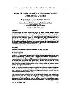
where the calls to f, h, p, q, g, and c actually indicate some arbitrary MRQL code (it does not matter what code it is as long as it does not depend on the query variables in a way other than the arguments shown). We can see that there are 7 query variables bound in the 5 select-expressions in the query: x, y, z, w, n, m, and k. There is no reason to construct an evaluation plan that produces a flat tuple (x,y,z,w,n,m,k) for each combination of the values of these variables that satisfies the join conditions, as is done in relational databases, because then we would have to group-by this stream to reflect the query nesting and to form the query answer, as it was done for the previous nested query. Instead, we want to construct an evaluation plan that delivers the data in a stream of tuples already grouped into the form ( x, y, {z}, {( w, n, {m} )} ), which reflects the query nesting directly and satisfies all the join conditions in the query. That is, each combination of x and z from the set {z} in such a tuple satisfies z.B=x.B, each y is from the set x.D and satisfies x.A=y.A, etc. Note that we should not include the variable k in the tuple because the domain of n is an expression that contains a select-query and has to be evaluated completely before we derive values for n. This special query domain that contains a select-query is called a nested domain query, and must be treated specially, as we will show next. The shape of the grouped variable values is described by a tree, called the query pattern tree, which is a kind of data type. Our framework uses one query pattern tree for each nested domain query, plus one

s

level 0

B

x

A

w

m

C

µn

C

x y

zs z

w n

A

level 1

ws ms

ks

level 2

B

z

y

C

K

G G

m

k

µy

k

level 3

A

n

B

µm W

X

Z

Figure 1: The pattern trees (A), the query graph (B), and the query plan (C) of the example query for each outer query. Thus, for the example query, there are two query pattern trees, one for the nested domain query of n and another for the entire query itself. These trees, which are depicted in Figure 1.A, are s(x,y,zs(z),ws(w,n,ms(m))) and ks(k) in prefix form. Each internal node in the pattern tree is associated with a selectquery. For example, the root s is associated with the outermost select-query. If internal nodes are taken to be sets of tuples, then the query pattern tree describes the required nesting of query variables concisely. If the input data is grouped in a way that reflects the query pattern tree, resulting to a set s (the root of the pattern tree), then the query can be evaluated over s using the function: header(s) = select f (select h(z) from z in zs) from (x,y,zs,ws) in s where p(select g(w,n) from (w,ms) in ws where c(select m.F from m in ms))

which is called the query header. The query header is derived from the query by associating a new query variable to each selectexpression in the query, by removing all the join and filter predicates, and by replacing the from-part of each select-expression with a single binding that uses a tuple pattern to bind the from-part variables and the query variables of the immediate nested selectexpressions. These bindings correspond to the nodes of the query pattern tree. They ungroup the grouped values in s, feeding the variable values to the appropriate nested queries. For the second pattern tree, which corresponds to the nested domain query for the variable n, the query header is: header2(ks,w) = g(select w.M+k.N from k in ks)

The next task is to generate the grouped values from the input data. The grouped data fed to the query header are generated by a join/unnest plan, which is derived from the query graph. The query graph represents all potential joins and unnests in the query concisely. We say that a variable v, defined by a binding v in e, depends on a variable w, if e refers to the variable w. The query graph is a graph whose nodes are query variables, the arrows are the variable dependencies, and the edges between the nodes v and w are equi-join conditions of the form f (v) = g(w), where f (v)/g(w) are expressions that depend on v/w. For our example query, the query graph is shown at Figure 1.B.

6.3 Deriving an Algebraic Form The next step is to derive an evaluation plan from the query graph, as the one shown at Figure 1.C for the graph in Figure 1.B, where ⊲⊳ is our algebraic join operator and µ is our cmap operator. The evaluation plan must deliver the data to the query header in groups that satisfy the join conditions and match the query pattern tree s(x,y,zs(z),ws(w,n,ms(m))) .

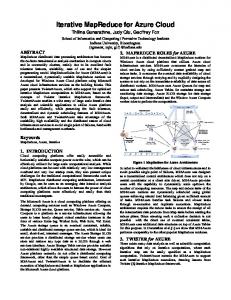
To synthesize a good plan from the query graph to evaluate the query, we use a polynomial heuristic algorithm, which we first introduced in the context of relational queries [12], but adapted here to work with nested queries and dependent joins. It is a greedy bottom-up algorithm, similar to Kruskal’s minimum spanning tree algorithm. This algorithm assumes that we know all the input sizes and the predicate selectivities in advance. If the graph reduction is done incrementally at run-time, by immediately executing the chosen operation from the query graph, then the sizes of the input data sources, as well as the sizes of the intermediate results, can be derived from the file system. The predicate selectivities though, which allow us to select the next graph reduction step and choose the best operation, can only be estimated using statistics. In our current system, which has an incomplete cost model, we set the selectivities to constants. Every node in the graph (which corresponds to a query variable) is assigned an estimated size, which is the size of the variable domain, and every edge (an equi-join predicate) is assigned an estimated selectivity. Each graph node may also be associated with a number of attributes, such as a filtering condition and a sort order. More specifically, each node i in the graph is associated with a query variable vi and a domain ri . Each node i is labeled with the size of ri , the physical algorithm used to derive ri , and other attributes associated with ri . Each edge between i and j is labeled with the selectivity Sij of the join predicate between i and j. The graph algorithm constructs the physical operator tree by merging graph nodes in pairs, as shown in Figure 2.A. At each step of the algorithm, we select two nodes i and j that do not depend on other nodes and have a minimum cost, and we merge them into a new node ij. The estimated cost to consider when we choose a pair of nodes depends on the join algorithm used, the sizes size(ri ) and size(rj ), the selectivity Sij , and the various attributes. The new size of ij is size(ri ) × size(rj ) × Sij and its operator is ri ⊲⊳ rj , where ⊲⊳ is annotated with the actual physical join algorithm with the least cost. In addition, for each node k connected to both i and j, the weight of the edge between k and ij becomes Sik × Sjk . Another graph simplification step to consider is depicted in Figure 2.B. It applies when a node j depends on one or more nodes i, which in turn should not depend on any variables. Then, j is merged with all these nodes i and the resulting node is associated with a cmap. We continue this process until we are left with only one node, which contains the final physical plan. At each graph reduction step, when a new plan operator (a join or a cmap) is assigned to the new node, the reduce function of this operator must be derived. The reduce function is composed in such a way that the plan operator takes a step towards grouping the data in the way specified by the final query pattern tree, that is, so that it delivers the data to the query header in groups that satisfy the join con-

size(ri ) ri

size(rj )

Sij

i Sik rk

j

ri

rj

ij

rj

i

µ j ij

k

Sij

A

size(rk)

size(ri )

size(ri )* size(rj)* Sij

Sik * Sjk

Sjk

k

size(ri )* size(rj)* Sij

rk

k

k size(rj )

size(rk)

j m

B m

Figure 2: The Query Graph Simplification Steps: A) generate a join or B) generate an unnest ditions and match the query pattern tree s(x,y,zs(z),ws(w,n,ms(m))) . For example, the X ⊲⊳ Z in the query plan in Figure 1.C is: join( λx. x.B,λz. z.B, λ(xs,zs). cmap(λx. {(x,zs)}) xs ) ( X, Z )

where the X input matches the pattern tree s(x) and the Z input matches the pattern tree zs(z) and the output is grouped by z that matches the pattern tree s(x,zs(z)).

6.4 Algebraic Optimization As it was previously discussed, MRQL group-by queries are translated to plain MRQL queries that contain calls to the groupBy operation. Each groupBy call requires the reduce task of a dedicated MR job. Given that Step 3 generates joins and cmaps from the query graph, the plans derived from that step consist of cmap, groupBy, and join operations. Before we translate these operations to our physical algorithms, we can optimize them even further by applying algebraic rewriting techniques to fuse cascaded operations, to minimize the number of required MR jobs, and to eliminate redundant operations. The most important optimization is to fuse two cascaded cmaps into a single cmap: cmap(f) (cmap(g) S) = cmap (λx. cmap(f) (g(x))) S

that is, instead of two cascaded cmaps, which require two MR jobs, we derive a nested cmap, which requires only one MR job (the inner cmap is evaluated in memory). Cmaps can also be fused with joins: cmap(m) (join(kx,ky,r) (X,Y)) = join( kx, ky, λ(xs,ys). cmap(m)(r(xs,ys)) ) (X,Y) GroupBy operations can be translated to MapReduce operations

using Eq. (1): cmap(r) (groupBy(cmap(m) S)) = MapReduce(m, r) S

If either or both cmap(m) or cmap(r) are missing, then we can always set m(x) = {x} or r(x) = {x}. Joins can be directly mapped to MapReduce2 operations using the rule: join(kx , ky , r)(X, Y ) = MapReduce2( λx.{(kx (x), x)}, λy.{(ky (y), y)}, r )

( X, Y ) The reason that MapReduce2 is more general than join is to allow map operations in the MapReduce2 inputs to be fused with the MapReduce2 operation at the physical level, thus requiring one MR job only. For example, we can use the rule: MapReduce2( mx , my , r )( cmap(f ) X, Y ) = MapReduce2( λv. mx (f (v)), my , r )( X, Y )

The fragment-replicate join MJoin, on the other hand, is more restricted than join since it must apply the reduce function at the map-

per one-element-at-a-time: join(kx , ky , λ(xs, ys). cmap(λx. r(x, ys)) xs)(X, Y ) = MJoin(kx , ky , r)(X, Y )

that is, a join is translated to an MJoin plan only when its reduce function has a certain shape. As described in Section 1 through the PageRank example, a MapReduce2 self-join can be rewritten into a simple MapReduce operation that traverses the input dataset once: MapReduce2( mx, my, r ) ( X, X ) = MapReduce( λz. cmap(λ(k,x). {(k,(1,x,null))}) (mx(z)) ∪ cmap(λ(k,y). {(k,(2,null,y))}) (my(z)), λ(k,s). r( cmap(λ(n,x,y). if n=1 then {x} else {}) s, cmap(λ(n,x,y). if n=2 then {y} else {}) s ) ) X

This transformation is similar to the semantics of join given in Section 5. Another transformation used in the PageRank example, is fusing a group-by with a join if the group-by key is the same as the join key: MapReduce2( λ(k,x). {(k,ex)}, my, r ) ( groupBy(X), Y ) = MapReduce2( λ(k,z). {(k,(k,z))}, my, λ(xs,ys). r(cmap(λx. {ex}) (groupBy(xs)),ys) ) ( X, Y ) It applies when the left MapReduce2 map function returns the groupby key k as the left join key, that is, when it looks like λ(k,x). {(k,ex)} for some expression ex.

6.5 Synthesizing the Combine Function The reduce function r of MapReduce(m, r) S must take the form r(k, s) = code, where s is a bag that contains all the elements associated with this key k and code is the body of the function. If the only use of variable s inside the code is in calls to either aggr(s) or aggr(cmap(f ) s), for some aggregations aggr and some functions f , then we can use the MapCombineReduce(m, c, r) S operation instead of MapReduce. To do so, we let the mapper generate the values aggr(f (x)) only, the combiner generate the values aggr(s) only, and all occurrences of aggr(cmap(f ) s) in the reducer code to be replaced with aggr(s). For multiple aggregations, variable s will be a tuple that contains the partial results of all these aggregations. Note that the avg (average) aggregation must be replaced with the sum divided by the count before this method is applied. For example, in the following operation MapReduce(λ(k,x). {(x.A,x)}, λ(k,s). {(k,sum(cmap(λx. {x.B}) s))}) X the aggregation sum(cmap(λx. {x.B}) s) is the only operation that accesses the group values s in the reducer. Based on our algorithm,

this operation can be transformed to: MapCombineReduce(λ(k,x). {(x.A,x.B)}, λ(k,s). {(k,sum(s))}, λ(k,s). {(k,sum(s))}) X since sum(f (x)) = sum({x.B})=x.B .

40

60 MRJ JG-MRJ

20

opt no-opt

40 30 20

15

10

5

10

opt no-opt

35

Total Time (minutes)

Total Time (minutes)

Total Time (minutes)

50

30 25 20 15 10 5

0

4 8 12 16 20 4 8 12 16 20 4 8 12 16 20 (GB) 8 nodes 6 nodes 4 nodes (A) TPCH nested query: MapReduce2 join (MRJ) vs join/group-by (JG) 60

8 6 4 (nodes) (C) PageRank over the Hungarian Web with/without optimization

8 6 4 (nodes) (B) PageRank over DBLP data with/without optimization

70 opt no-opt

140 opt no-opt

40

30

20

120

Total Time (minutes)

60

Total Time (minutes)

50

Total Time (minutes)

0

0

50

40

30

opt no-opt

100 80 60 40

20 20

10

10 0

2

4

6

8

10

RMAT-i dataset (x10^6 nodes, x10^7 edges) (D1) PageRank over RMAT on 8 nodes with/without optimization

0

2

4

6

8

10

0

RMAT-i dataset (x10^6 nodes, x10^7 edges) (D2) PageRank over RMAT on 6 nodes with/without optimization

2

4

6

8

10

RMAT-i dataset (x10^6 nodes, x10^7 edges) (D3) PageRank over RMAT on 4 nodes with/without optimization

Figure 3: Query Evaluation over (A) TPCH, (B) DBLP, (C) the Hungarian Web, and (D1-D3) RMAT-i graphs

7.

PERFORMANCE EVALUATION

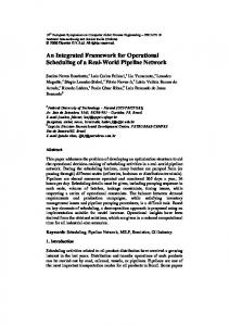
MRQL is implemented on top of Hadoop. The source code is available at http://lambda.uta.edu/mrql/. Currently, our system can evaluate any MRQL query over XML, JSON, binary, and record-oriented text documents (with basic values separated by user-defined delimiters). The platform used for our evaluations was a small cluster of nine Linux servers (circa 2006), connected through a Gigabit Ethernet switch. The cluster was managed by Rocks Cluster 5.4 running CentOS-5 Linux. For our experiments, we used Hadoop 0.20.2, distributed by Cloudera. The cluster frontend was used exclusively as a NameNode/JobTracker, while the rest 8 compute nodes were used as DataNodes/TaskTrackers. Each server has 4 Xeon cores at 3.2GHz with 4GB memory. That is, there were a total of 32 cores available for map/reduce tasks. We repeated our experiments for 3 different Hadoop configurations: 8 nodes (32 cores), 6 nodes (24 cores), and 4 nodes (16 cores). For each configuration, we had to format the DFS and reinstall the data to make sure that data blocks were equally distributed to data nodes. Our first measurement evaluates the effectiveness of our optimization techniques for nested queries, which use our generalized join that incorporates data nesting. For this experiment, we used the Orders and Customer tables from the TPCH benchmark. We used 5 datasets TPCH-i, for i = 1, . . . , 5, of size i ∗ 4GBs (the total size of Orders and Customer tables) using the TPCH dbgen option -s = i ∗ 20. That is, the largest dataset was 20GBs. We considered the following MRQL query: select c.NAME from c in Customer where avg(select o.TOTALPRICE from o in Orders where o.CUSTKEY=c.CUSTKEY) < 150000.0

which selects the customers whose average order prices are below 150K. MRQL translates this query to a single MapReduce2 join. Using traditional optimization techniques, we could have generated a flat join followed by a group-by. Figure 3.(A) compares the

graph = select ( key, select x. to from x in n ) from n in source(line , "graph.csv" ,...) group by key: n.id ; size = count(graph); select (x. id , x.rank) from x in (repeat nodes = select < id: key, rank: 1.0/size, adjacent: al > from (key,al ) in graph step select (< id : m.id, rank: n.rank, adjacent: m.adjacent >, abs((n.rank−m.rank)/m.rank) > 0.1) from n in (select < id : key, rank: 0.25/size+0.85∗sum(select x.rank from x in c) > from c in ( select < id : a, rank: n.rank/count(n.adjacent) > from n in nodes, a in n.adjacent ) group by key: c.id ), m in nodes where n.id = m.id) order by x.rank desc;

Figure 4: PageRank in MRQL

evaluation time of this query using the MapReduce2 join, called MRJ, versus the evaluation time based on the traditional method of using a join (a simplified MapReduce2) followed by a groupby with aggregation (a MapCombineReduce), called JG. The histograms shown in Figure 3.(A) show the MRJ time (white boxes) and the time difference JG-MRJ (shaded boxes). We can see that, for all three cluster sizes (4, 6, and 8 nodes), the time improvement using our joins was between 50% and 65%, thus justifying our decision for using a special join for nested queries. The next query we evaluated was PageRank over various datasets. The complete PageRank query is given in Figure 4. Given that our datasets represent a graph as a flat list of edges, the first query in Figure 4 groups this list by the edge source so that each tuple in the resulting graph contains all the neighbors of a node in a bag. We only measured the execution time of the last query in Figure 4, which calculates the PageRank of the graph (this is done by the repeat MRQL expression) and then orders the nodes by their rank.

Recall from Section 3 that, for the repeat to converge, the condition abs((n.rank-m.rank)/m.rank) > 0.1 must become false for all graph nodes. The purpose of this evaluation was to measure the effectiveness of the algebraic rewrite rules for fusing a join with a group-by and for mapping a self-join to a MapReduce that traverses the input once (these rules are described informally in Section 1 and formally in Section 6.4). The optimized query requires one MapReduce per iteration, while the non-optimized query requires one MapReduce2 and one MapReduce per iteration. We evaluated PageRank with and without these optimizations over the following datasets: 1. DBLP: the DBLP dataset in XML format, available at http://dblp.uni-trier.de/xml/, which is 865MBs. The citation graph we considered had 1.7M papers and 112K citations. PageRank required 10 steps to converge. 2. HG: the Hungarian web graph http://web-graph.org/, which is 734MBs, has 500K nodes and 14M links. PageRank required 9 steps to converge. 3. RMAT-i: synthetic data generated by the R-MAT algorithm [9] using the parameters a=0.57, b=0.19, c=0.19, and d=0.5 for the Kronecker graph generator. The number of distinct edges generated were 10 times the number of nodes. We used 10 datasets RMAT-i, for i = 1, . . . , 10, of size i∗140MBs, with i ∗ 106 nodes and i ∗ 107 edges. That is, the largest dataset was 1.4GBs. PageRank required 6 steps to converge. Figures 3.(B) and 3.(C) show the evaluation of PageRank over the DBLP citation graph and over the Hungarian Web for a cluster of 8, 6, and 4 nodes. From Figures 3.(D1)-(D3), we can see that there is no clear winner for the synthetic graphs generated by R-MAT. If there are enough nodes to assign tasks or less data (more precisely, when the number of available cores is at least 50% more than the number of data blocks), then our optimizations clearly win. This suggests that a cost-based optimizer must consider both plans and choose the best based on data size and system resources.

8.

CONCLUSION AND FUTURE WORK

We have presented an SQL-like query language that is expressive enough to capture most map-reduce computations. We have also presented an algebra, physical plan operators, and an effective optimization framework that identifies opportunities for joins and translates every query construct to map-reduce operations in Hadoop. The most important component that needs to be completed and improved in our framework is a comprehensive cost model based on statistics. In the future, we are planning to use a dynamic cost analyzer, where statistics are collected and the optimization is done at run-time. More specifically, we are planning to develop a method to incrementally reduce the query graph at runtime, and enhance the reduce stage of a map-reduce operation to generate enough statistics to decide about the next graph reduction step. In addition, the Hadoop map-reduce operation uses a number of parameters that need to be adjusted for better performance, such as the number of reducers. We are planning to investigate techniques for incorporating these parameters into the cost model. Acknowledgments: This work is supported in part by the National Science Foundation under the grant 1117369.

9.

REFERENCES

[1] A. Abouzeid, et al. HadoopDB: An Architectural Hybrid of MapReduce and DBMS Technologies for Analytical Workloads. In VLDB’09.

[2] S. Babu. Towards Automatic Optimization of MapReduce Programs. In SOCC’10. [3] D. Battre, et al. Nephele/PACTs: A Programming Model and Execution Framework for Web-Scale Analytical Processing. In SOCC’10. [4] A. Behm, V. Borkar, M. J. Carey, et al. ASTERIX: Towards a Scalable, Semistructured Data Platform for Evolving-World Models. Distrib Parallel Databases (2011) 29: 185–216. [5] V. Borkar, M. J. Carey, R. Grover, N. Onose, and R. Vernica. Hyracks: A Flexible and Extensible Foundation for Data-Intensive Computing. In ICDE’11. [6] Y. Bu, B. Howe, M. Balazinska, and M. D. Ernst. HaLoop: Efficient Iterative Data Processing on Large Clusters. In VLDB’10. [7] M. J. Cafarella and C. Re. Manimal: Relational Optimization for Data-Intensive Programs. In WebDB’10. [8] R. Chaiken, et al. SCOPE: Easy and Efficient Parallel Processing of Massive Data Sets. In PVLDB’08. [9] D. Chakrabarti, Y. Zhan, and C. Faloutsos. R-MAT: A Recursive Model for Graph Mining. In SDM’04. [10] J. Dean and S. Ghemawat. MapReduce: Simplified Data Processing on Large Clusters. In OSDI’04. [11] J. Dittrich, et al. Hadoop++: Making a Yellow Elephant Run Like a Cheetah (Without It Even Noticing). In VLDB’10. [12] L. Fegaras. A New Heuristic for Optimizing Large Queries. In DEXA’98. [13] L. Fegaras, C. Li, U. Gupta, and J. J. Philip. XML Query Optimization in Map-Reduce. In WebDB’11. [14] A. F. Gates, et al. Building a High-Level Dataflow System on top of Map-Reduce: the Pig Experience. In PVLDB 2(2), 2009. [15] Hadoop. http://hadoop.apache.org/. [16] M. Isard, M. Budiu, Y. Yu, A. Birrell, and D. Fetterly. Dryad: Distributed Data-Parallel Programs from Sequential Building Blocks. In EuroSys’07. [17] M. Isard and Y. Yu. Distributed Data-Parallel Computing Using a High-Level Programming Language. In SIGMOD’09. [18] E. Jahani, M. J. Cafarella, and C. Ré. Automatic Optimization for MapReduce Programs. In PVLDB’11, 4(6). [19] S. P. Jones and P. Wadler. Comprehensive Comprehensions (Comprehensions with Order by and Group by). In Haskell’07. [20] J. Lin and C. Dyer. Data-Intensive Text Processing with MapReduce. Book pre-production manuscript, April 2010. [21] MRQL. http://lambda.uta.edu/mrql/. [22] C. Olston, B. Reed, U. Srivastava, R. Kumar, and A. Tomkins. Pig Latin: a not-so-Foreign Language for Data Processing. In SIGMOD’08. [23] R. Pike, S. Dorward, R. Griesemer, and S. Quinlan. Interpreting the Data: Parallel Analysis with Sawzall. Scientific Programming 13(4), 2005. [24] M. Stonebraker, et al. MapReduce and Parallel DBMSs: Friends or Foes? In CACM 53(1), 2010. [25] A. Thusoo, et al. Hive: a Warehousing Solution over a Map-Reduce Framework. In PVLDB 2(2), 2009. [26] A. Thusoo, et al. Hive: A Petabyte Scale Data Warehouse Using Hadoop. In ICDE’10. [27] T. White. Hadoop: The Definitive Guide. O’Reilly, 2009. [28] H.-C. Yang, A. Dasdan, R.-L. Hsiao, and D.S. Parker. Map-Reduce-Merge: Simplified Relational Data Processing on Large Clusters. In SIGMOD’07.