Juan Blanch, Alex Ene, Todd Walter, Per Enge. Stanford University. ABSTRACT ...... the ION GNSS 2005, Long Beach, CA, September 2004. [13] Oehler, V.
An Optimized Multiple Hypothesis RAIM Algorithm forVertical Guidance Juan Blanch, Alex Ene, Todd Walter, Per Enge Stanford University
ABSTRACT For several years, Receiver Autonomous Integrity Monitoring (RAIM) has been used successfully for horizontal positioning in the phases of flight with Protection levels on the order of several hundreds of meters. In the next years, there will be many more navigation satellites (Galileo, a renewed GLONASS constellation, Compass), all expected to have signals in at least two frequencies. This has raised the possibility of using RAIM for much more demanding phases of flight (LPV 200 or Cat. I, for example), and perhaps ultimately replacing integrity providers such as SBAS and GBAS. However, it is not possible to apply the assumptions that are made for RAIM today in studies for vertical approach availability. Among others, the definition of failure needs to be changed: because the expected accuracy will be better, the threshold for failure will be reduced; as a consequence, the prior probability of failures could be larger than what is used now. This, together with the fact that there will be many more ranging sources makes it necessary to consider the possibility of multiple simultaneous failures. There are several RAIM algorithms treating multiple failures. However, most of them present certain disadvantages: either the calculations required to compute the Protection Levels are very complex, or the link between these Protection Levels and the Probability of Hazardously Misleading Information is problematic (often because several approximations are necessary). In this paper, we give a detailed explanation of an optimized Multiple Hypothesis Solution Separation algorithm for RAIM. There are several advantages in the Multiple Hypothesis approach. First, the link between threat model, Protection Level and PHMI is a very easy and straightforward one; second, the calculation of the Protection Level does not involve complex steps. We will show how these advantages stem mostly from the fact that the algorithm works by computing a Protection Level that meets the PHMI requirement, rather than computing a probability of misdetection. One of the key points in this algorithm is the allocation of the PHMI to the different failure modes. In previous papers, the allocation was made heuristically, in this one we will show how to compute an optimal allocation. As an example, the
algorithm will be applied to a single dual frequency constellation (GPS or Galileo) and a dual constellation.
INTRODUCTION In the next years, several GNSS constellations are expected to become operative, such that users will have access to a large number of pseudoranges in two frequencies, which will allow receivers to cancel the ionosphere induced error. This has raised the possibility of using RAIM to provide worldwide coverage of vertical guidance (starting with LPV 200), with a reduced need for ground monitoring [1], [2], [3]. However, compared to the algorithms used currently for horizontal positioning, the RAIM algorithms will need to be updated such that they accommodate complex threats (in particular multiple failures with any number of satellites and different a priori probability of failure), have a rigorous proof of safety (Probability of Hazardously Misleading Information) while not being unnecessarily conservative. Generalizations of the slope based RAIM algorithm [5] to multiple failures have been devised [6], however the threat model is not clearly defined and the proof of safety still relies on approximations. The algorithm presented here is an improvement on the algorithm that has been described in [1], which in turn is a modification of the Multiple Hypothesis Solution Separation algorithm described in [4]. Also, the algorithm is bears several similarities with other RAIM algorithms based on solution separation [5]. The main features of the optimized MHSS RAIM algorithm are as follows. First, as long as one can provide a definition of the threat and an a priori probability, the algorithm can account for it. In particular, multiple failures with an arbitrary number of satellites can be included in a transparent way. Second, the algorithm has a simple proof of safety: the Probability of Hazardously Misleading Information (HMI) is computed by adding up the contribution of each failure, following a fault tree (as it is done in the Wide Area Augmentation System proof of safety [7]). Finally, The Probability of HMI is allocated dynamically to increase performance (by reducing the Protection Levels). Dramatic gains in
performance can be obtained in the case of heterogeneous a priori probability of failure for different fault modes
but not on the pseudorange errors. interpretation that will be adopted here.
The paper starts by defining the threat model framework and describing the baseline MHSS RAIM algorithm. Then, the optimization of the integrity budget allocation is explained - the original contribution of this paper. After that, we present a little-known formula linking slope based RAIM and solution separation RAIM. This formula allows us to compare slope based RAIM with solution separation RAIM. Finally, the optimized algorithm is used to assess the global coverage of vertical guidance using RAIM with high prior probabilities of failure.
The PHMI can be computed by counting the contribution of each possible error model state weighted by its prior probability:
THREAT MODEL The threat model is defined here as a collection of error model states that partition the whole space. A probability is associated to each error model state (or fault mode), which corresponds to the a priori probability of being in a given state i, which is labeled Pap,i. Typically, such collection of states includes a nominal mode which has a probability close to one. For the examples developed in this paper, each state corresponds to a partition of the measurements between nominal measurements (measurements that follow a known nominal distribution) and faulty measurements (measurements that are not tied to a distribution, and in particular, that could “conspire” against users). Therefore, if there are n measurements, there are at most 2n error model states. In the nominal state, the pseudorange error is assumed to be overbounded (in the sense of [9], for example) by a Gaussian distribution with a maximum bias. In the examples used in the results, it is assumed that the satellite failures are independent with probability Psat. As a consequence the probability of failure of a given satellite is Psat, the probability of failure of a given set of two satellites is Psat2, etc. Notice, that this is a conservative approximation, since the probability of failure of one satellite and one only is slightly smaller than Psat. However, the difference is small with the values of Psat used here.
DEFINITION OF PROBABILITY OF HAZARDOUSLY MISLEADING INFORMATION The Probability of Hazardously Misleading Information (PHMI) is the probability that the true position lies outside the error bound determined by the user. As it was pointed out in [8], this definition is not complete as it does not specify on what the probability is conditioned on. The usual interpretation of this probability is that it is conditioned on the geometry and the error characteristics,
PHMI =
N states
∑P
ap , i
i =1
This is the
P ( HMI | i )
Notice that it is not necessary to identify the correct error state model. It is only necessary to compute an error bound such that the true position is within the bound with sufficient probability.
BASIC ALGORITHM The main idea of the approach is to compute as many position solutions as there are possible error model states (subsets of failed satellites). For each solution, a subinterval around it is computed (corresponding to nominal errors). Then, an interval is formed such that all sub intervals are included in it. If these sub-intervals are chosen carefully, then it is possible to show that the probability of the true solution being outside this interval is below the required PHMI. Real time First, a list of all error models is tabulated. The maximum number of the error models is equal to the number of subsets of satellites that is 2n. The PHMI budget, labeled PHMIreq is distributed among all the modes. For the basic algorithm, the determination of each term is arbitrary: PHMI req =
N mod −1
∑ i =0
PHMI i
Next, for each mode, a vertical position solution and a sub-interval is computed such that:
(
)
P xv( i ) − xv ≥ L( i ) | i ≤
PHMI i Pap ,i
Both xv(i) and Li are computed by using only the nominal measurements in the error model i (thus ignoring the measurements that are arbitrary). Let us assume that state 0 corresponds to the failure free case. The real time Vertical Protection Level (VPL) associated to the all in view position is given by:
(
VPLRT = max xv(i ) − xv( 0) + Li i
)
VPL= max ( M i + Li ) i
Proof of safety The interval defined by this VPL and the all in view position is such that: ⎡ xv(i ) − Li , xv( i ) + Li ⎤ ⊂ ⎡ xv(i ) − VPLRT , xv(i ) + VPLRT ⎤ ⎦ ⎣ ⎦ ⎣
As a consequence:
EXAMPLE
(
)
PHMI i i i P ( HMI | i ) ≤ P xv( ) − xv ≥ L( ) | i ≤ Pap ,i
And:
PHMI =
N mod
∑ P ( HMI | i )P
ap ,i
i =0
≤
N mod
∑ i =0
PHMI i Pap ,i = PHMI req Pap ,i
Predicted VPL The algorithm described in the previous paragraphs computes the real time error bound. As one can see from the definition of the real time VPL, this depends on the actual measurements. (Notice that the probability that is computed is the system probability, not the probability conditioned on the measurements). In many applications, an upper bound of the error bound VPLRT needs to be predicted with a specified probability, labeled Pcont here (for continuity). That is, we need to determine VPL such that:
P (VPLRT > VPL ) ≤ Pcont
(
P (VPLRT > VPL ) = P ∃i | xv( ) − xv( ) + Li ≥ VPL ≤
∑ i =1
(
i
0
P xv( ) − xv( ) + Li ≥ VPL i
Here we give an example of the application of the algorithm which covers many practical applications. Let us suppose that there are n pseudorange measurements. The geometry matrix is labeled G. The pseudorange errors have a nominal error characteristic well described by a Gaussian distribution with standard deviation σk and maximum bias bk. A weighting matrix W is defined by: ⎡σ 12 0 0 ⎤ ⎢ ⎥ W =⎢ 0 % 0 ⎥ ⎢ 0 0 σ n2 ⎥ ⎣ ⎦
−1
Each failure is characterized by a partition of the measurements in nominal and failed. Let us consider one failure mode, which is indexed as i. A geometry matrix Gi is defined that has the same size as G but with zeros in the rows corresponding to the (possibly) faulty measurements. It is assumed that more than 4 rows are non zero, so that a position can be computed. Real time VPL
The definition of VPLRT gives:
N mod −1
With this definition, the continuity requirement is met. It is important to notice that this framework is extremely flexible: As long as one can compute the position and error bound in the known presence of each threat, the VPL can be derived.
0
)
)
Again, the continuity budget Pcont is distributed among all the modes (although not the all-in-view mode):
In real time, we can compute xv(i) for each mode as a linear combination of the measurements that are not affected by the fault:
xv(i ) = h(i ) y A good choice for h is given by: h(i ) = [ 0 0 1 0] ( GiT WGi ) GiT W −1
N mod −1
∑ i =1
Pcont ,i = Pcont
For each mode we determine Mi such that in nominal conditions:
(
)
P xv( i ) − xv( 0) ≥ M i ≤ Pcont ,i
It is assumed here that the 3rd component is the height. Let us define: −1
k =1
Then Li can be defined as: The VPL is then defined as:
n
σ v2,i = h( i )W −1h( i )T = ( GiT WGi )3,3 and Bv ,i = ∑ hk(i ) bk
Li = K PHMI ,iσ v ,i + Bv ,i
In this equation, KHMI,i is defined as:
⎛ PHMI i ⎞ K HMI ,i = Q −1 ⎜1 − ⎟ ⎜ 2 Pap ,i ⎟⎠ ⎝ With this definition, the PHMI requirement is met.
-
Predicted VPL In order to compute a predicted VPL, we need to compute the terms Mi, which bound the expected separation between the different solutions.
(
P xv( ) − xv( i
0)
) ( (h
≥ Mi = P
(i )
− h(
0)
)y ≥M ) i
As this is the predicted solution separation under nominal conditions, its distribution is overbound by a normal distribution with standard deviation σss,i and bias Bss,i: B
(
)
(
σ ss2 ,i = h( i ) − h( 0) W −1 h(i ) − h( 0)
)
T
and
n
Bss ,i = ∑ hk(i ) − hk( 0) bk i =1
In the Appendix, it is shown that in the case that W is diagonal we have the relationship:
σ ss2 ,i = σ v2,i − σ v2,0
the weighted least squares solution based on the weighting matrix. Other weights might provide a smaller error bound, in particular if biases are on the same order of magnitude as the random errors [SOCP reference] the continuity budget (or false alarm probability) allocation the PHMI budget allocation
In this algorithm it is not possible to optimize the allocation given the measurements themselves, as the proof of safety assumes that an allocation is made before the measurements are known. The allocation cannot be dependent on the measurements. The search of optimal subset solution coefficients is independent for each mode, and independent of the allocations. Once this choice has been made, we can associate a function to each subset solution i: ⎛ PHMI i VPLi ⎜ Pcont ,i , ⎜ Pap ,i ⎝
M i = K cont ,iσ ss ,i + Bss ,i
The constant Kcont,i is defined by: ⎛ P ⎞ K cont ,i = Q −1 ⎜ 1 − cont ,i ⎟ 2 ⎠ ⎝
OPTIMIZATION
In the previous section, the baseline algorithm has been described, along with a general example. In this section, the method to optimize the VPL is described, which is the original contribution of this work. First, it is necessary to understand over which variables one can optimize. It is possible to vary: -
the set of coefficients used for each subset solution. In the previous example, we have used
⎞ ⎟⎟ ⎠
As was described earlier, the final VPL is obtained by taking the maxima of the VPLi, so that the problem of minimizing the VPL can be formulated as: ⎛ ⎛ PHMI i Minimize max ⎜ M i ( Pcont ,i ) + Li ⎜ ⎜ P i ⎜ ⎝ ap ,i ⎝ N mod −1
Subject to The term Mi can be defined as:
⎞ ⎛ PHMI i ⎟⎟ = M i ( Pcont ,i ) + Li ⎜⎜ ⎠ ⎝ Pap ,i
∑ i =1
Pcont ,i = Pcont and
N mod −1
∑ i =0
⎞⎞ ⎟⎟ ⎟ ⎟ ⎠⎠
PHMI i = PHMI
The optimal solution to this problem is unknown to the authors of this work. However, because both Li and Mi are decreasing functions of their arguments, one can show that at the minimum all the VPLi are equal. A simple proof is as follows: suppose that one of the terms is above the remaining ones, one could increase the allocation of that term (and decrease the other ones) so that the net effect would be a reduction in the VPL. This is a useful property that suggests strategies that, although suboptimal, produce better results than an arbitrary allocation. Before describing how the minimization was done in this work, we indicate how to compute a lower bound on the VPL. It is possible to evaluate a lower bound of the optimal VPL (which we don’t know how to calculate) by evaluating: ⎛ ⎛ PHMI i Minimize max ⎜ M i ( Pcont ) + Li ⎜ ⎜ P i ⎜ ⎝ ap ,i ⎝
⎞⎞ ⎟⎟ ⎟ ⎟ ⎠⎠
N mod −1
∑
Subject to
i =0
PHMI i = PHMI
The difference here is that each mode is allocated the full continuity budget. Because Pcont is usually on the order of 10-6, optimizing the continuity budget does not decrease the VPL substantially: the ratio between the sigma containment at 10-6 to the sigma containment at 10-7 is less than 10%, and the continuity term is usually less than 50% of the total VPL, such that the total decrease is less than 5%. It is due to this reason that in this work, the continuity budget was allocated arbitrarily (which determines Mi) whereas the integrity was allocated optimally. Once the continuity budget has been allocated, the problem to solve is of the form: Minimize max ( fi ( xi ) ) i
N mod −1
Subject to
∑ i =0
xi = PHMI
where fi are decreasing functions. As indicated above, at the minimum we have:
(
fi xi(
min )
) = f ( x( ) ) = L 0
min 0
So the problem can be reformulated as: Minimize L N mod −1
Subject to
∑ i =0
fi −1 ( L ) = PHMI
This is a mono-dimensional problem that can be easily solved numerically, for example by interval halving.
ADDITIONAL CONSIDERATIONS
Extension to the horizontal dimension The algorithm can be extended to the horizontal dimension using the same approach that is used in the WAAS Horizontal Protection Level calculation [10]. For Gaussian errors, it is not straightforward to compute the probability of a horizontal error being below a certain threshold. It is however easy to find an overbound by finding the direction of maximum error (corresponding to the maximum eigenvalues of the covariance in the horizontal plane) and using Rayleigh statistics instead of Gaussian statistics [10].
The bias also needs to be accounted and an overbound of the bias in any direction in the horizontal plane needs to be computed. It is proven in the Appendix that the maximum bias in the horizontal plane for a given a set of coefficients S and maximum pseudorange biases can be bounded by:
max ( u T Sb ) ≤
∑
u =1 u ⊥ vertical
2
+
S1, k bk
k
∑
2
S 2, k bk
k
In this equation, it is assumed that the dimensions corresponding to the horizontal plane are the first one and the second one. Exclusion The algorithm presented here computes the Protection Level once the measurements are dimmed to be consistent. It is important to keep in mind that exclusion is not an integrity issue: leaving a corrupt measurement in the solution will simply degrade the Protection Levels such that a given service is not available. An exclusion algorithm well adapted to a Multiple Hypothesis Solution Separation algorithm has been described in [1]. However, any exclusion method can be used in conjunction with the algorithm presented here. Continuity error bounds and integrity error bounds In the examples shown above, the same nominal error models have been used for both the integrity part of the VPL and the continuity part. It is possible to use a different set of models for continuity and integrity. The integrity model error needs to be an overbounding density for each given user. The continuity error model can be averaged over different users and conditions (although for the same geometry). For this reason, the continuity bounds are not as stringent as the integrity bounds. For each pseudorange, two additional parameters are introduced here to describe the continuity error bound: σcont,k and bcont,k. The continuity parameters are used in the formulas for σss,i and Bss,i: B
Wcont
(
2 ⎡σ cont 0 0 ⎤ ,1 ⎢ ⎥ 0 ⎥ =⎢ 0 % 2 ⎢ 0 ⎥ 0 σ cont ,n ⎦ ⎣
)
(
−1
−1 σ ss2 ,i = h( i ) − h( 0) Wcont h( i ) − h ( 0 ) n
Bss ,i = ∑ hk( i ) − hk( 0) bcont , k i =1
)
T
This approach allows users to compute less conservative predicted protection levels while meeting the integrity requirements in real time.
LINK WITH MAXIMUM SLOPE BASED RAIM
In this section we introduce as an aside a comparison between solution separation RAIM and chi-square based RAIM. This paragraph shows that while the two methods behave similarly, there are significant differences that can result in different performance levels. Link with maximum slope based RAIM For this section it will be assumed that: - Nominal biases are zero - There are n failure modes corresponding to each satellite failing at a time This last assumption is made here to lighten the notation, and the conclusions reached in this paragraph do not need it. In this paragraph the differences and common points of slope based RAIM and MHSS RAIM are highlighted. As opposed to MHSS RAIM, Maximum slope based RAIM only checks the chi-square statistic that can be formed from the residuals. One of the approaches of slope based RAIM is the one described in [weighted RAIM], which is summarized here. The methodology has been generalized to multiple failures in at least one way [Angus]. The formula for the VPL is given by:
VPL = max (Vslopek ) T + K md σ v ,0 k
For one line of sight, the slope is given by: hk( ) σ k 0
Vslopek =
Pkk
where P is defined by: P = W − WG ( G T WG ) G T W −1
The threshold T is set by the required false alarm probability. At first sight, this formula is appears to be very different from the MHSS formulation. However they are actually very similar since there is the exact relationship: Vslopek = σ ss , k = σ
2 v,k
−σ
(In this paragraph, we can use the same index k for both the mode and the line of sight.) The slope based VPL is defined by:
VPL = max (σ ss , k ) T + K md σ v ,0 k
Differences with slope based RAIM In slope RAIM the proof of safety relies on certain approximations [cite Brown] which are not proved to be conservative, but have been dimmed sufficient for large error bounds (such as for En Route, Terminal and LNAV). The main formula is obtained by assuming that all the errors are coming from the failed subset, and that the magnitude of the chi-square statistic is only a function of the bias of the failed subset. Ad hoc terms are added in two different ways to account for the effect of the nominal noise, but they are not strictly conservative. (However, if both terms are added, then it is strictly conservative). This is an important point when comparing the magnitude of the VPL using other methods. One can see the effect of this approximation in the second term of the VPL: whereas the MHSS solution uses the standard deviation of the subset, slope RAIM uses the standard deviation of the all-in-view set. Another drawback of slope RAIM is the loss of information that occurs when forming the chi-square statistic (instead of exploiting the residual vector, which has N-4 degrees of freedom.) This loss of information causes the difference in the first term of the VPL equation. The chi-square statistic threshold defines an ellipsoid (with degenerate dimensions). The first term of the VPL corresponds to the maximum solution separation given that the measurements fall within the ellipsoid. However, there are ample regions in the ellipsoid that do not result in a large solution separation. As a consequence, the use of the chi-square statistic as a discriminator, while practical, appears to be arbitrary. It is interesting to notice that once the whole vector of residuals is used (through the subset solutions), it is possible (and easy) to compute a provably conservative VPL. While it is not possible to directly compare the relative performances, we can compare the first term in the VPL by computing the ratio: T
2 v ,0
K cont ,i
=
χ n2− 4 −1 (1 − Pcont ) ⎛ P ⎞ Q −1 ⎜1 − cont ,i ⎟ 2 ⎠ ⎝
For the purposes of the comparison, we can choose to divide the continuity budget among the failure modes (a conservative factor of 3 is added here to account for the continuity allocation in the horizontal dimension): Pcont ,i =
Pcont 3 ( N mod − 1)
Performance evaluation
In Table 1, the resulting ratio is shown for n varying from 5 to 20 and n = Nmod and Pcont = 4 10-6. One can see that there is a clear advantage in using the solution separation statistic rather than the chi-square statistic. Nsat T
5 .96
8 1.12
11 1.23
14 1.31
17 1.39
20 1.46
K cont ,i
Table 1. Ratio between the first term in the VPL between a chi square based protection level and a solution separation based protection level.
In addition, to the performance considerations, MHSS RAIM allows a much more flexible threat model (varying a priori probability of failures, nominal biases, distinction between continuity and integrity error bounds).
RESULTS
To illustrate the optimized algorithm, we show availability and coverage results corresponding to a single constellation and a dual constellation (GPS and Galileo). The integrity nominal standard deviation σk is defined by: 2 σ k2 = σ URA + σ k2, DF _ air + σ k2,tropo
The continuity nominal standard deviation σcont,k is defined by: 2 2 2 2 σ cont , k = σ cont ,URA + σ k , DF _ air + σ k , tropo
The error models specifying the Code Noise and Multipath (CNMP) error bound and the tropospheric error are described in the Appendix. In addition we need to specify the User Range Accuracy both for integrity and continuity as well as the maximum bias. In all the performance evaluations we assume: -
Please refer to the section on Additional Considerations for the difference between the continuity and integrity error bounds. The required integrity (PHMI) and continuity (Pcont) requirements are 10-7 and 4 10-6 respectively.
σURA =.7 m (integrity) and σURA,cont = .25 m (continuity) Nominal bias b = 1 m (integrity) and continuity bias bcont = .1 m
The performance of the algorithm was evaluated by using the set of MATLAB scripts MAAST [11] to compute the predicted VPL of a set of users distributed over the world during one day. The users are placed on a grid every 5 degrees in both longitude and latitude (which gives 2592 locations). For each location, the geometries are simulated every 5 minutes (which gives 288 epochs). For each time and location a VPL is computed following the algorithm specified above. Comparison with a non-optimized MHSS RAIM algorithm In order to illustrate the benefits of the optimization, the algorithm is compared to a non-optimized MHSS algorithm. Notice however, that the non-optimized algorithm needs to be minimally modified to achieve sufficient performance: some of the low a priori probability fault modes with weak geometries can be excluded before ever computing the associated interval, because their probability is so small that they don’t need to be mitigated by the RAIM algorithm. Single constellation (27 satellites in three planes) The first example considers a three plane constellation with 27 satellites (one of the options considered for Galileo) [12]. The probability of failure per satellite is chosen to be 10-4. (which matches the probability of fault that is assumed in the Galileo Safety-of-life concept [13]). It will be assumed that the failures are independent, such that the probability of two simultaneous failures is 10-8. These need to be considered because the probability of any two failures is above the total integrity budget of 10-7. The VPL map is shown in Figure 1. The meaning of this map is the following: the value plotted is the 99.9 percentile of all the VPL values computed at a given location over the course of a day.
VPL as a function of user location 80 60
Average 99.9% VPL Coverage of 99.9% 20 m avail.
Latitude (deg)
40 20 0
Equal Allocation 18.6 m
Optimized Allocation 15.1 m
83.7%
100%
-20
Table 3. Performance summary for a single constellation with 27 satellites
-40 -60 -80 -150
-100
-50
0
50
100
Dual constellation
150
Longitude (deg) < 12
< 15
< 20
< 25
< 30
< 35
< 40
< 50
> 50
VPL (m) - 99.9%
Figure 1. 99.9 Percentile of the VPL over the course of a day for a single constellation.
In Table 2, we show the difference between the performance of the optimized algorithm compared to the non-optimized one. Although the average VPL reduction is about 15% only, the difference for the coverage of 35 m (with 99.9 % availability) is significant, since there with the optimized allocation algorithm there is no unavailability. Equal Allocation Average 99.9% VPL Coverage of 99.9% 35 m avail.
28.4
Optimized Allocation 24.2
95.5%
100%
Table 2. Performance summary for a single constellation with 27 satellites VPL as a function of user location 80
The second example considers a dual constellation with the Galileo (the same as in the first example) and a 24 satellite GPS constellation (the optimized 6 plane constellation defined in [10]). The probability of fault per satellite was chosen to be 10-3, which is a very high probability of failure. The resulting VPL map is shown in Figure 2 and the summary of results in Table 3. The reduction in average VPL is in this case close to 20%. The increase in the coverage of 20 m VPL (with 99.9 % availability) is dramatic: it goes from 83.7% to 100%.
CONCLUSION
The algorithm presented here is very flexible in the threat model it can protect against; also, its proof of safety relies on a PHMI calculation based on a fault tree (which is an accepted methodology for WAAS and LAAS); finally, it dynamically allocates the integrity budget among possible failure modes to optimize the Protection Levels. This dynamic allocation improves substantially the performance of the baseline MHSS RAIM algorithm (15% to 20% in VPL reduction), bringing the coverage to 100% in cases with high probabilities of satellite failure (10-4 for a single constellation with 27 satellites and as high as 10-3 for a dual constellation (27+24)).
60
Latitude (deg)
40
APPENDIX
20
Two-step Minimization
0 -20
Another possibility is to approach the optimization is by minimizing independently the continuity term (M) and the integrity term (L):
-40 -60 -80 -150
-100
-50
0
50
100
(
Minimize max M i ( Pcont ,i )
150
i
Longitude (deg)
N mod −1 < 12
< 15
< 20
< 25
< 30
< 35
< 40
< 50
Subject to
> 50
VPL (m) - 99.9%
Figure 2. 99.9 Percentile of the VPL over the course of a day for a dual constellation.
∑ i =1
And then:
)
Pcont ,i = Pcont
⎛ ⎛ PHMI i Minimize max ⎜ M i ( Pcont ,i ) + Li ⎜ ⎜ P i ⎜ ⎝ ap ,i ⎝ N mod −1
∑
Subject to
i =0
⎞⎞ ⎟⎟ ⎟ ⎟ ⎠⎠
Vslopei =
PHMI i = PHMI
Biases in the horizontal dimension We prove: max ( u Sb ) ≤
2
∑S
∑S
+
bk
1, k
u =1 u ⊥ vertical
k
2 2, k
bk
k
u T Sb = cos θ ∑ S1, k bk + sin θ ∑ S2, k bk k
∑S
≤ cos θ
k
b + sin θ
1, k k
k
∑S
k
2
+
b
1, k k
k
b
2
+
b
1, k k
∑S
b
1, k k
2
b
excluded. We have:
(
xˆ − xˆiˆ = G T WG
)
−1
(
GT Wy − GiˆT Wiˆ Giˆ
( G WG ) g w = 1 − g w ( G WG ) −1
T
i
T i
i
−1
T
i
)
−1
GiˆT Wiˆ yiˆ
( y − g (G WG ) g T i
i
T
−1
G T Wy
)
i
So that: var eT ( xˆ − xˆiˆ ) =
(
)
⎛ eT ( GT WG )−1 g w i i ⎜ ⎜ 1 − g T w G T WG −1 g ) i i i ( ⎝
2
⎞ 2 ⎟ E ⎛ y − g T ( G T WG )−1 G T Wy ⎞ i i ⎜ ⎟ ⎟ ⎝ ⎠ ⎠
⎛ eT ( G T WG )−1 g w i i =⎜ ⎜ 1 − g T w GT WG −1 g ) i i i ( ⎝
(
)
(
⎞ ⎟ ⎟ ⎠
2
E yi2 − 2 giT ( G T WG ) gi wi yi2 + giT ( G T WG ) g i −1
(e (G WG ) T
=
T
−1
g i wi
−1
)
2
wi − g wi ( G WG ) gi wi T i
)
= Vslopei2
T
−1
)
((G W G )
+
∑S
T iˆ
iˆ
iˆ
−1
− ( G T WG )
−1
)e
The proof is as follows:
(
E ( xˆ − xˆi )( xˆ − xˆi )
b
∑S
(
var eT ( xˆ − xˆiˆ ) = eT
k
2
b
∑S
b
2, k k
k
T
(
)
= E ( cov GT W − covi GT Wi ) yyT ( cov GT W − covi GT Wi )
T
= ( cov G T W − covi G T Wi ) W −1 ( cov GT W − covi GT Wi )
T
2, k k
k
1, k k
k
∑S
2, k k
2, k k
k
≤
∑S
2
k
∑S
b
2, k k
k
∑S
+
wi − wi g iT cov g i wi
iˆ mean that the pseudorange (or set of pseudoranges) is
We also have:
b
1, k k
∑S
=
Pii
k
∑S
≤
eT cov g i wi
In this equation, the vector e is the direction of the coordinate of interest. The matrices with the subscript
As pointed out earlier the benefit of optimizing over the continuity allocation is much smaller than the benefit of optimizing the integrity allocation. Also, it can be very damaging to performance, because some modes with very weak geometries have a disproportionate effect on the final bound, even though they might have a very low a priori and could have been excluded in the first place. The equal allocation of the continuity allows some terms to be very large, but when the PHMI allocation is optimized, those terms are effectively canceled (the PHMI allocation to these modes matches the a priori of the fault.)
T
hi
2
b
2, k k
k
= cov − cov GT Wi G covi − covi G T Wi G cov+ covi GT WiW −1Wi G covi = cov + covi − cov GT Wi G covi − covi GT Wi G cov
Formulas relating Solution Separation RAIM and slope based RAIM The formula for the slope used in weighted RAIM is the following:
G T Wi G = cov i−1
Finally, we have:
(
E ( xˆ − xˆi )( xˆ − xˆi )
T
) = cov − cov i
So that:
σ ss2 ,i = σ v2,i − σ v2,0 = Vslopei2
)
Besides linking the two main forms of RAIM, this last formula provides an easy way to compute the generalized slope term that was described in [6].
[5] Brown, R. G., “A Baseline GPS RAIM Scheme and a Note on the Equivalence of Three RAIM Methods”, Navigation, v.39, no.3, 1992.
Nominal Error Models Here is the definition of the Code Noise and Multipath (CNMP)error and tropospheric error used in the Results section. The CNMP error bound is given by: ⎛
[4] Pervan, B., Pullen, S. and Christie, J., “A Multiple Hypothesis Approach to Satellite Navigation Integrity”, Navigation, v.45, no.1, 1998.
2
2
⎛ f2 ⎞ f12 ⎞ 2 σ L1, k , air + ⎜ 2 5 2 ⎟ σ L25, k , air 2 2 ⎟ ⎝ f1 − f 5 ⎠ ⎝ f1 − f5 ⎠
σ k2, DF _ air = ⎜ where:
σ L21, k , air = σ L25, k , air = σ k2, noise + σ k2, multipath f1 and f5 are the L1 and L5 frequencies. The multipath contribution is defined in [10] for AAD-A aircraft:
σ k , multipath = 0.13 m + ( 0.53 m ) e −θ 10° The noise term was assumed to be: σ k , noise = 0.04 m − ( 0.02 m )(θ k − 5° ) / ( 85° ) This formula was taken from [14].
[6] Angus, J. “RAIM with Multiple Faults”. Navigation, v.53, no.4, 2006. [7] Fernow, J.P. “WAAS Integrity Risks: Fault Tree, “Threats”, and Assertions” http://www.faa.gov/about/office_org/headquarters_offices /ato/service_units/techops/navservices/gnss/library/briefin gs/media/IWG/Integrity_risks_fault_tree_threats_assertio ns_rev3.ppt. [8] Blanch, J., Walter, T., Enge, P. “Understanding PHMI for Safety of Life Applications.” Proceedings of the Institute of Navigation's National Technical Meeting, San Diego CA, 2007.
k
The tropospheric error is assumed to be bounded by: ⎛ ⎞ 1.001 ⎟ σ k ,tropo = ( 0.12 m ) ⋅ ⎜ ⎜ 0.002001 + sin 2 ( Elk ) ⎟ ⎝ ⎠
ACKNOWLEDGEMENTS
This work was sponsored by the FAA GPS Satellite Product Team (AND-730). REFERENCES
[1] Ene, A., Blanch, J., Powell, J.D., “Fault Detection and Elimination for Galileo-GPS Vertical Guidance,” Proceedings of the Institute of Navigation's National Technical Meeting, San Diego CA, 2007. [2] Lee, Y.C., Braff, R., Fernow, J.P., Hashemi, D., McLaughlin, M.P., and O’Laughlin, D., “GPS and Galileo with RAIM or WAAS for Vertically Guided Approaches”, Proceedings of the ION GNSS 2005, Long Beach, CA, September 2005. [3] Nikiforov, I., Roturier, B., “Advanced RAIM Algorithms: First Results”, Proceedings of the ION GNSS 2005, Long Beach, CA, September 2005.
[9] Rife, J., Pullen, S., Pervan, B., and Enge, P. “Paired Overbounding and Application to GPS Augmentation” Proceedings of the IEEE Position Location and Navigation Symposium, Monterey, CA, April 2004. [10] WAAS Minimum Operational Standard, RTCA SC 159 DO-229C. [11] S. S. Jan, W. Chan, T. Walter, P. Enge. “Matlab Simulation Toolset for SBAS Availability Analysis,” Proceedings of the Institute of Navigation GPS-01, Salt Lake City, 2001. [12] Zandbergen, R., Dinwiddy, S., Hahn, J., Breeuwer, E., Blonski, D., “Galileo Orbit Selection”, Proceedings of the ION GNSS 2005, Long Beach, CA, September 2004. [13] Oehler, V., Trautenberg, H.L., Luongo, F., Boyero, J.-P., Lobert, B., ”User Integrity Risk Calculation at the Alert Limit without Fixed Allocations”, Proceedings of the ION GNSS2005, Long Beach, CA, September 2004. [14] Murphy, T. et al. “Results from the Program for the Investigation of Airborne Multipath Errors.” Proceedings of the Institute of Navigation's National Technical Meeting, San Diego CA, 2005.