An Online-Optimized Incremental Learning Framework for Video Semantic Classification Jun Wu
1
Xian-Sheng Hua, Hong-Jiang Zhang
Bo Zhang
Department of Computer Science and Technology, Tsinghua University Beijing 100084, P. R. China
Microsoft Research Asia, 5F Sigma Center, No.49 Zhichun Road Beijing 100080, P. R. China
Department of Computer Science and Technology, Tsinghua University Beijing 100084, P. R. China
[email protected]
{xshua; hjzhang}@microsoft.com
[email protected]
ABSTRACT This paper considers the problems of feature variation and concept uncertainty in typical learning-based video semantic classification schemes. We proposed a new online semantic classification framework, termed OOIL (for Online-Optimized Incremental Learning), in which two sets of optimized classification models, local and global, are online trained by sufficiently exploiting both local and global statistic characteristics of videos. The global models are pre-trained on a relatively small set of pre-labeled samples. And the local models are optimized for the under-test video or video segment by checking a small portion of unlabeled samples in this video, while they are also applied to incrementally update the global models. Experiments have illustrated promising results on simulated data as well as real sports videos.
Categories and Subject Descriptors H.3.1 [Information Storage and Retrieval]: Content Analysis and Indexing-indexing methods; I.2.10 [Artificial Intelligence]: Vision and Scene Understanding-video analysis.
General Terms Algorithms, Experimentation.
Keywords Incremental Learning, Video Analysis, Concept Drifting, Video Semantic Classification
1. INTRODUCTION Structure analysis is an elementary step for mining the semantic information in videos, among which semantic classification of video segments are essential for further content analysis, as well as important for enabling semantic-level video retrieval. In human being’s understanding, semantic concept is relatively clear and easy to identify, while due to the large gap between semantics and low-level features, the corresponding features are generally not concentrated in feature space. This is an open difficulty for typical computer vision and content analysis issues. Many related technologies have been reported in literature ([1] to [6], [11]) to address the issue of video semantic classification, which generally can be classified into two categories, rule-based methods and learning-based methods. Permission to make digital or hard copies of all or part of this work for personal or classroom use is granted without fee provided that copies are not made or distributed for profit or commercial advantage and that copies bear this notice and the full citation on the first page. To copy otherwise, or republish, to post on servers or to redistribute to lists, requires prior specific permission and/or a fee. MM’04, October 10–16, 2004, New York, New York, USA. Copyright 2004 ACM 1-58113-893-8/04/0010…$5.00.
Rule-based approaches utilize domain knowledge to design specific rules for semantic classification. Generally, rule-based methods are difficult to capture all the rules manually, as well as have limited generalization capacity. And semantic concept “drifting”, which frequently happens in video analysis, may completely destroy a well-built rule-based system. Learning-based methods use statistic machine learning algorithms to model the semantic classes (generative learning) or the discrimination of different classes (discriminative learning). In [2], hidden Markov model and dynamic programming are applied to play/break segmentation. Fan et al [11] classify semantic concepts for surgery education videos with Bayesian classifiers by using an adaptive EM algorithm. Zhong et al [4] proposed a unified framework for scene detection and structure analysis by combining domain-specific knowledge with supervised machine learning methods. As a whole, most of learning-based approaches require sufficient training data to achieve good generalization capacity, and almost all of them are only capable of doing offline classification. However, due to the large data size of videos, typically video related learning problems are always lack of training data, compared with the relatively large variations of video semantic concepts. Nevertheless, it is observed that though the semantic concept has large variations and keep drifting in feature space, they are locally consistently distributed. That is, the variation within one video or video segment is relatively much smaller than that among different videos. We call this property “Time Local Consistency”, as “within a video or video segment” actually means that the content is close in timeline. Furthermore, though the semantic concept is drifting, its drifting speed is relatively slow, which means the concept is drifting gradually along the timeline. This phenomenon is termed as “Concept Drifting Gradualness” here. Though we should say this observation might not always be true, it is nearly satisfied for many applications. Based on above observations, we proposed a novel online semantic classification framework, termed OOIL (for OnlineOptimized Incremental Learning), in which two sets of optimized classification models, local and global, are online trained by sufficiently exploiting both local and global statistic characteristics of videos. The primary advantages of this framework are in threefold. Firstly, only a relatively small number of pre-labeled training samples are required at initial stage, which tackles the issue of lacking in training samples in typical video applications. Secondly, the applying of online (locally) optimized models deals with the issue of feature variation when the system is in an “immature” state, as well as the issue of overfitting when the system is in a relatively “mature” state. Thirdly, the framework is applicable for real time applications (with a short period of delay). 1
This work is performed when the first author was a visiting student in Media Computing Group, Microsoft Research Asia.
The remainder of this paper is organized as follows. In Section 2, the online-optimized incremental learning framework is presented. Experiments are introduced in Section 3, followed by conclusion remarks and future works in the Section 4.
defining a given mixture. Typical EM algorithm will iteratively maximize maximum likelihood (ML) to estimate Θk,c based on the training samples yc as Θˆ = arg max L(Θ , y ) (2) k ,c
2. ONLINE-OPTIMIZED INCREMENTAL LEARNING (OOIL) FRAMEWORK Suppose the feature vector (random variable) for identifying a certain set of specific semantic concepts is denoted by Y = [Y(1), Y(2), …, Y(d)]T, where d is the dimension of the feature vector, with y = [y(1), y(2), …, y(d)] T representing one particular outcome of Y. The set of training samples for semantic concept c (1≤ c ≤ C) is denoted by yc = {y1,c, y2,c, …, yn(c),c} (n(c) is the number of labeled samples for concept c). And the (unlabeled) samples of the under-test video, ordered by timestamp, are represented by x = {x1, x2, …, xT}. Figure 1 shows the flowchart of our proposed online-optimized incremental learning framework, which consists of three primary modules: Global Model Pre-Training (GMPT), Local Adaptation (LA) and Global Incremental Updating (GIU). …
Training Samples of Class 1 y1
…
GMM 1
GMM C
GMPT
Local GMM
Local GMM 1
AEM x( t): First portion of x
Global GMM 2
…
…
Local GMM C
Global GMM C
Classification
As aforementioned, semantic concepts have a so-called “Time Local Consistency” property, which enlightens us to improve the classification accuracy by exploring the characteristics of certain amount of the unlabeled samples in current under-test video.
{
k −1
k
}.
(3)
Local adaptation is to find a set of local GMMs which are the combinations of the global GMM models represented by { Θ k ( c ),c , 1 ≤ c ≤ C }, and Θ t t , aiming at optimizing the classification k
performance on current under-test video, i.e., x.
Output
Figure 1. Online-optimized incremental learning framework. In this framework, firstly C GMM models (termed Global GMM Models) are generated by training on the pre-labeled training samples using a so-called Agglomerative EM (AEM) algorithm [8]. Then for the under-test video, the first portion (say, 10 minutes) is also modeled by a GMM using AEM algorithm. Thereafter, this GMM is compared with all the Global GMM Models, to generate C local optimized GMM models which are then applied to classify the under-test video samples. At last, all the Global GMM Models are updated by combining the local optimized models and the original global models. And, these updated global models will be used for the next test video. The details of this framework are presented as follows.
2.1 Global Model Pre-Training As mentioned above, firstly, pre-labeled training samples are used to train a set of Global GMM Models by AEM algorithm [8]. Suppose a certain semantic concept c has a finite mixture distribution in feature space Y, represented by
(
2.2 Local Adaptation (Optimization)
k
LA
) ∑ α m ,c N ( µ m , c , Σ m ,c )
f Y y c | Θ k ,c =
Denote k(c) the best k obtained from AEM, and then the optimal GMM, represented by the optimal parameters, is Θk(c),c (for simplicity, the hat “ ˆ ” on the optimal parameters are omitted).
Θ t t = θ1t , θ2t ,L, θ t t , α1t , α 2t ,L, α t t
GIU Under-test Samples x
To estimate best k=k(c) for yc, typically Minimum Description Length (MDL) criterion is applied. In this paper, a modified EM algorithm, AEM, which is based on Mixture MDL (MMDL) [8], is adopted to estimate Θk,c and k for the global GMM models from the labeled samples.
Global GMM 1
Local GMM 2
c
Let x(t) = {x j, 1≤ j ≤ t, t ≤ T } be the first portion of x, the (unlabeled) samples of the under-test video. Similar to pretraining process in above sub-section, we estimate a GMM for the sample set x(t). Suppose the estimated GMM parameters are denoted by
Training Samples of Class C yC AEM
AEM
k ,c
Θ k ,c
k
(1)
m =1
where k is the number of components, N (µm,c, Σm,c) is an Gaussian component, θm,c = (µm,c, Σm,c) is its mean and covariance matrix, and αm is the mixing probabilities ( ∑m =1 α m,c = 1 ). Let Θk,c= k
{ θ1,c, θ2,c, … , θk,c, α1,c, α2,c, … , αk-1,c} be the parameter set
As aforementioned, the semantic concept may drift gradually over time. GMM local adaptation is designed to reduce the affection caused by concept drifting by locally adapting GMM models on a small portion of the under-test video samples, as following steps. Step 1: Compute the symmetric Kullback-Leibler (KL) divergence (distance) [9] (Ds) of every pair of Guassian components in the models represented by Θ k ( c ),c and Θ t t , as below form
(
k
(
D s (c, i, j) = D s N (y c | µ i,c , Σ i,c ), N x(t ) | µ tj , Σ tj
(
)( )
⎞⎤ − Σ i,−c1 ⎟ ⎥ (4) ⎠⎦ T⎡ −1 ⎤ 1 + µ i,c − µ tj ⎢ Σ i,−c1 + Σ tj ⎥ µ i,c − µ tj 2 ⎦ ⎣ Step 2: Compute the distance between each semantic concept c and each Gaussian component in Θ t t , defined by =
1 ⎡ ⎛ tr Σ i,c − Σ tj ⎜ Σ tj 2 ⎢⎣ ⎝
))
(
)
−1
( ) (
)
k
D(c, j ) = min D(c, i, j )
(5)
1≤ i ≤ k ( c )
t
t
Let J (c) be a subset of {1, …, k }, defined by
{
}
J t (c ) = j : c = arg min D (s, j ) .
(
1≤ s ≤C
)
(6)
Step 3: Gaussian components N x(t )| µ tj , Σ tj , j ∈ J t(c), are taken
as a new GMM estimation of semantic concept c for the under-test video samples. That is, the local GMM for the certain semantic concept c is
⎞⎟ = f X ⎛⎜ x | Θ l l k ( c ) ,c ⎠ ⎝
∑t
j∈J (c)
α tj α (c ) l
(
)
N µ tj , Σ tj ,
(7)
where α l (c) = ∑ j∈J t ( c ) α j , kl(c) = | J t(c) | is the number of Gaussian components in the localized GMM. Therefore, for a sample xi in the under-test video, the classification result is determined by ⎞⎟⎫ . c (x i ) = arg max ⎧⎨ f X ⎛⎜ x i | Θ l l (8) ⎬ k ( s ),s ⎠ ⎭ 1≤ s ≤C ⎩ ⎝ That is, the sample xi is classified to semantic concept c (x i ) .
2.3 Global Model Incremental Updating In this step, we introduce the scheme for updating the global GMM models by combining the original global models with the localized models. The updated models will be applied as global models for new upcoming videos, thus, the “concept drifting” in previously tested videos are “kept” in the updated global models, which will affect the classification results of new videos. For convenience, the localized GMM for concept c is represented by ⎞⎟ = f X ⎛⎜ x | Θ l l k ( c ),c ⎠ ⎝
k l (c )
∑α lj,c N (µlj,c , Σ lj,c ) .
(9)
j =1
To update the global GMMs, we combine the components in original GMMs with the most “close” ones in the localized GMMs, or add new components to the global models, as follows.
(
)
Step 1: For each Gaussian component N µlj,c , Σ lj,c in localized GMM
Θl l k (c),c
, find the most “close” component N ( µi,c , Σ i,c ) in
Θ k ( c ),c by comparing Kullback-Leibler divergences (DKL) [9] as
( (
)
)
i = arg min D KL N µ lj,c , Σ lj,c , N ( µ m,c , Σ m,c ) . 1≤ m≤ k(c)
(10)
If the minimum DKL in (10) is larger than a predefined threshold, go to Step 2’ (adding new components). Otherwise, go to Step 2 (adjusting existing components). Step 2: Gaussian component N ( µi,c , Σ i,c ) in global GMM Θ k ( c ),c is replaced by N µ*i,c , Σ i,*c , which is defined by
(µ
* * i,c , Σ i,c
)=
(
)
(
(
) (
arg min DKL (1 − α ) N (µi,c , Σ i,c ) + α N µ lj,c , Σ lj,c , N µ*i,c , Σ i,*c ( µ ,Σ )
)) , (11)
where α is a parameter standing for the updating “speed”. According to reference [10], µ*i,c , Σ i,*c has a close form as
(
)
µ*i,c = (1 − α ) µi,c + α µlj,c ,
(
)
( ) ⎞⎟⎠ − µ (µ ) . (13)
Σ i,*c = (1 − α ) Σ i,c + µi,c µi,Tc + α ⎛⎜ Σ lj,c + µ lj,c µ lj,c ⎝
(
)
(12) T
* i,c
* i,c
T
Step 2’: N µlj,c , Σ lj,c is added into Θ k ( c ),c as a component, and ′ +1,c has the form of the updated global Gaussian model Θk(c)
(
)
k
f Y y c | Θ k (c )+1,c = ∑ (1 − β )α m,c N(µm,c , Σ m,c ) + β N '
m =1
(
µ lj,c , Σ lj,c
),
(14)
where β is also a parameter controlling the updating “speed”.
3. EXPERIMENTS To evaluate the proposed OOIL framework, we compare it with a number of related schemes or the same scheme but under different settings both on simulated data and real sports videos.
3.1 Schemes for Comparison As we have presented, the OOIL framework has three major features, i.e., effectively utilizing unlabeled samples in under-test videos, GMM local adaptation (LA), and global GMM incremental updating (GIU). Experiments are designed to evaluate the effectiveness of each feature, as well as any possible combination of them. Accordingly, four frameworks (8 cases in total, as some frameworks have different settings) are designed as follows. A. OOIL framework Except for the proposed version of OOIL scheme detailed in Section 2 (denoted by A1), two modified versions are derived: A2 - OOIL but using updated global models for classification: Compared with A1, the online updated global GMM models are employed for online classification. A3 - OOIL without GIU: Compared with A1, GIU step is skipped. B. Training only using labeled samples B1 - Training global models offline: A set of pre-labeled samples are utilized to train global models, which are then used to classify all other test videos (i.e., it is a commonly used learning process). B2 - Online training with “increasing” labeled data set: Both the set of initial pre-labeled global training samples and the samples on all previously classified videos (manually labeled too) are utilized to train new global models, which are used to classify next upcoming video. Obviously this scheme utilizes more training information than A1-A3 and B1, which generally is not practical in real applications. However, we will show that our proposed scheme (A1) can achieve close performance as this scheme but only using much less training data. C. Online training using both labeled and unlabeled samples C1: Similar to B2, while the training samples from the have-tested videos are not manually labeled, but labeled by the classification results using the global models (thus this portion of labeled samples may contain noise). C1 has the same training data as A1-A3, but uses different model updating method. We will show the model updating method in A1-A3 is better than this one. D. Allow checking “labeled” data D1: Similar to A1 (recall it stands for the proposed scheme), except the local models are obtained directly from the first portion of current under-test video which is manually labeled, instead of using unlabeled samples by LA which is presented in Section 2.2. Obviously, this scheme uses more training data than A1-A3, B1, B2, and C1. We will show that the performance of the proposed scheme (A1) is close to that of this scheme, but without using any labeled samples from the current under-test video. D2: Similar to D1, except there are no global models. That is, for each under-test video, only the first portion of the samples in it is applied to train local models which are used to classify this video.
3.2 Testing on Simulated Data As illustrated in Figure 2 (a), the simulated data consists of six groups denoted by D(t), 0 ≤ t ≤ 5, and each group has two classes, denoted by G1(t) and G2(t) (12000 samples for each class). They are drawn from two 3-component Gaussian mixture models, by gradually shifting the center of the Gaussian components along time t. The gray items represent G1(t) and the white items G2(t). More precisely, the GMM models are defined by ⎡0.2
α j = 1 / 3 , µ j = [ X gj , t , Y gj, t ]T , Σ j = ⎢ ⎣0
0⎤ ⎥, 0.2⎦
where 1 ≤ j ≤ 3 is the component number, g = 1, 2 is the class number, t is the group number, and ⎧ X gj , t = 7 + K g cos(π − tπ / 10) + 0.7 cos( jπ / 3 − π / 6) ⎪ ⎨ j K g sin(π − tπ / 10) + 0.7 sin( jπ / 3 − π / 6) ⎪⎩ Yg , t =
⎛ ⎧ K1 = 4 ⎞ ⎟ ⎜⎨ ⎜ K2 = 7 ⎟ . ⎠ ⎝⎩
2rp/(r+p) vs. t ( eight schemes ) 1
D = {G1,G2}
0.9
t=5 G2(t)
t=3 t=2 t=1
t=0
G1(t)
2rp/(r+p)
t=4 0.8
0.7 0.6
0.5 1
A1,D2 A2,D1 A3 B1 B2 C1 2
3 4 Group Index : 1 ≤ t ≤ 5
5
Figure 2. (a) Distribution of the simulated data (Left). (b) The performance (along timeline) of different schemes on simulated data set (Right). The first group (t = 0) is used as initial training data for global models, and other five sequential groups (t = 1 to 5) are treated as test data set. For the schemes requiring samples from current under-test data, the first 2000 samples are used. The above eight schemes of the four frameworks are performed to execute classification tasks and the results are illustrated in Table 1 (left). We use an evaluation measure “RP”, defined by 2rp/(r+p) (as described in [7]), where p means precision and r recall, which are computed upon the whole test data set. Table 1. Performance evaluation results of the eight schemes. A1 A2 A3 B1 B2 C1 D1 D2
p 0.994 0.995 0.729 0.627 0.993 0.679 0.995 0.994
Simulated data r RP 0.994 0.994 0.981 0.988 0.989 0.840 1.000 0.771 0.975 0.984 1.000 0.809 0.981 0.988 0.994 0.994
p 0.954 0.967 0.954 0.960 0.955 0.962 0.961 0.958
Sports videos r 0.927 0.900 0.927 0.785 0.806 0.788 0.936 0.941
RP 0.940 0.931 0.940 0.863 0.874 0.866 0.948 0.949
From this table, it can be concluded that: (1) Using local models obtained by LA step achieves slightly better performance than using global models after GIU step for the OOIL framework (A1 vs. A2). (2) Though only using a portion of unlabeled samples in the under-test data group, our OOIL framework successfully obtains local adapted models through LA, and achieves the same performance as the schemes that allow using labeled data of current under-test groups (as D1 and D2). (3) Compared with the common training scheme (B1: RP=0.771), global models are updated to enhance the performance in three ways: GIU described in Section 2.3, which is the best one (A1: RP=0.994), retraining by increasing training data set (B2: RP=0.984), or retraining upon the set of labeled samples plus previously classified samples (C1: RP=0.809). Furthermore, comparing the RPs of A1 and A3 (0.994 vs. 0.840), it also can be seen that GIU step significantly improves the performance. In addition, the classification performances for different test data groups are illustrated in Figure 2 (b). It can be concluded that the performances of the schemes without using GIU or LA (as A3, C1, and B1) decrease dramatically when the test data drifts.
3.3 Testing on Real Sports Videos Totally five baseball videos (about 15 hours) are applied in this experiment. The aforementioned eight learning schemes are employed to detect “pitch view” [4], and the results are shown in Table 1 (right). The training and testing samples are sampled (one by five) frames from these videos. Each sample is manually labeled as pitch view or non-pitch view frame. Similar to the experiments on simulated data, the samples from the first two videos are taken as initial training samples. Totally, there are about 37280 real instances of pitch view in the test set. For the schemes requiring samples from current under-test video, the samples from the first 10 minutes are used. The block-wise grass and sand ratios are applied as classification features (each frame is divided to 4×4 blocks, thus the feature dimension is 32=4×4×2). From Table 1 (right), we can draw similar conclusions as testing on simulated data, except that GIU step does not achieve such significant improvement for the proposed OOIL framework (A1 vs. A3). This can be explained that the concept drifting on this data set is not as evident as it on the simulated one.
4. CONCLUSION AND FUTURE WORK In this paper, we have proposed a new online video semantic classification framework, in which two sets of optimized models, local and global, are online trained by sufficiently exploiting both local and global statistic characteristics of videos. The global models are pre-trained on a relatively small set of pre-labeled samples. While the local models are optimized for the under-test video by checking a small portion of unlabeled samples in this video, which are also applied to incrementally update the global models. Furthermore, this framework can be applied to real time classifications, and only requires a small number of initial training samples, as well as the model localization and updating strategies tackle both the issue of large feature variation and over-fitting. Future work would be to theoretically develop an optimal model merging strategy for the previous global models and localized models, as well as test the framework on larger video database, more types of videos, and more semantic concepts.
5. REFERENCES [1] P. Xu, et al, Algorithms and Systems for Segmentation and Structure Analysis in Soccer Video, ICME2001, pp 22-25.
[2] L. Xie, et al, Structure Analysis of Soccer Video with Hidden Markov Models, ICASSP 2002, Vol 4, pp 13-17.
[3] Y.Gong, T.S. Lim, and H.C. Chua, Automatic Parsing of TV Soccer Programs, ICMCS 1995, pp 167-174.
[4] D. Zhong, S-F. Chang, Structure Analysis of Sports Video Using Domain Models, ICME 2001, pp 713 -716.
[5] G. Sudihir, J.C.M. Lee, A.K. Jain, Automatic classification of tennis [6] [7] [8] [9] [10] [11]
video for high-level content-based retrieval, IEEE Intl Workshop on CBAIVD 1998. Baoxin Li, et al, Event Detection and Summarization in Sports Video, IEEE Intl Workshop on CBAIVL 2001. S. Raaijmakers, et al, Multimodal topic segmentation and classification of news video, ICME 2002, Vol 2, pp 33-36. M. Figueiredo, et al, On Fitting Mixture Models, Energy Minimization in Computer Vision and Pattern Recognition, E. Hancock and M. Pellilo (Eds.), Springer-Verlag, 1999. S. Kullback, Information Theory and Statistics, J. Wiley & Sons, New York, 1959. M. West, J. Harrison, Bayesian Forecasting and Dynamic Models, Springer Verlag, New York, 1989. Jianping Fan, et al, Semantic video classification by integrating flexible mixture model with adaptive EM algorithm, ACM SIGMM MIR 2003, pp 9-16.