Sep 9, 2006 - For a given number of particle size bins, the isogradient scheme significantly .... deposition as simulated using a classical size bin scheme.
Click Here
JOURNAL OF GEOPHYSICAL RESEARCH, VOL. 111, D17310, doi:10.1029/2005JD006797, 2006
for
Full Article
An optimized particle size bin scheme for modeling mineral dust aerosol G. Foret,1 G. Bergametti,1 F. Dulac,1,2 and L. Menut3 Received 21 October 2005; revised 24 February 2006; accepted 2 May 2006; published 9 September 2006.
[1] During transport, atmospheric aerosol particles experience nonlinear size-dependent
deposition processes which affect their size distribution. This implies that the aerosol particle size distribution (PSD) should be well represented in three-dimensional transport models that simulate their transport and their radiative or biogeochemical impacts. In particular, mineral dust aerosols exhibit a broad range of particle sizes but the dust PSD is generally described in such models by a limited number of particle size bins. A common approach in the literature consists in defining such bins following a geometric progression of the particle diameter (‘‘isolog’’ bins). Here we propose to define size bins following the size dependence in dry deposition velocity (Vd), by satisfying an ‘‘isogradient’’ in Vd. We use a box model and reference simulations with 1000 particle size bin to test the accuracy of both approaches with 4 to 30 bins, in simulating (1) the mineral dust number and mass PSD evolution due to dry and wet deposition, and (2) the derived visible aerosol optical thickness (AOT). Both schemes show a trend in increasing accuracy when increasing the number of bins. The classical isolog scheme, however, exhibits strong, embarrassing oscillations in accuracy when varying the number of bins. For a given number of particle size bins, the isogradient scheme significantly improves the accuracy of results in terms of mass PSD and greatly suppresses oscillations of errors in both mass and number distributions. We conclude that at least eight isogradient size bins are necessary to secure an 8% accuracy on the total suspended dust mass after two days of transport. In terms of particle number distribution, errors remain small for both schemes but they become somewhat larger (�8%) in terms of AOT for 12–30 isogradient size bins. This drawback can be compensated by weighting the average aerosol extinction cross section within each size bin by the initial dust particle number distribution. We conclude that at least eight isogradient size bins are necessary. Citation: Foret, G., G. Bergametti, F. Dulac, and L. Menut (2006), An optimized particle size bin scheme for modeling mineral dust aerosol, J. Geophys. Res., 111, D17310, doi:10.1029/2005JD006797.
1. Introduction [2] Soil-derived dust is one of the major tropospheric aerosol components [Intergovernmental Panel on Climate Change (IPCC), 2001]. Owing to the large masses of mineral material injected from arid and semiarid surfaces by wind in the atmosphere, dust is a key species of many biogeochemical cycles [Swap et al., 1992; Jickells et al., 2005]. Atmospheric dust deposition supplies seawater of open oceans with terrigeneous elements, many of them (Fe, P. . .) being suspected to be limiting nutrients [Bergametti et al., 1992; Duce, 1995; Falkowski et al., 1998]. Dust is also considered to play a significant role in the Earth energy budget by absorption and 1 Laboratoire Interuniversitaire des Syste`mes Atmosphe´riques, Universite´s Paris 7 & 12, UMR CNRS 7583, Cre´teil, France. 2 Laboratoire des Sciences du Climat et de l’Environnement, UMR CNRS-CEA-UVSQ 1572, Commissariat a` l’Energie Atomique, Saclay, France. 3 Laboratoire de Me´te´orologie Dynamique, Ecole Polytechnique, UMR CNRS 8539, Palaiseau, France.
Copyright 2006 by the American Geophysical Union. 0148-0227/06/2005JD006797$09.00
scattering. Owing to their large size spectrum, dust particles affect both the incoming solar radiation flux and the longwave outcoming emission of the Earth [Sokolik and Toon, 1996; Sokolik et al., 2001]. Neither the sign nor the intensity of the dust radiative forcing is, up to now, precisely assessed [IPCC, 2001]. Finally, dust archives from deep ocean sediments, ice cores, lakes or continental loess deposits are used as proxies of past environmental and climate conditions [Petit et al., 1990; Grousset et al., 1992; Rea, 1994]. Thus dust remains one of the most challenging species to model in order to understand, evaluate and predict biogeochemical cycles and climate changes. [3] When looking to existing dust measurements in the atmosphere or dust transport as seen by satellites, we observe that the variability in time and space of dust concentration is very high. Indeed, dust is only emitted when the wind velocity exceeds a threshold value and the dust source strength is roughly proportional to the third power of the wind velocity [Bagnold, 1941; Gillette, 1979; Marticorena and Bergametti, 1995]. Thus their emissions are sporadic both in frequency and intensity. Moreover, dust is present in many different sizes, with particle diameters
D17310
1 of 15
D17310
FORET ET AL.: OPTIMIZED BIN SCHEME FOR MODELING DUST
ranging from about a tenth up to several tens of microns [d’Almeida and Schu¨tz, 1983; Gomes et al., 1990]. This leads to a special sensitivity of the dust cycle to size dependent processes occurring during atmospheric transport, like dry and wet deposition, with an impact on dust interactions with radiation. [4] First global dust aerosol models considered a unique aerosol particle size [e.g., Joussaume, 1993], a limited number of constant modes (e.g., 4 size bins with their respective size distribution assumed constant in the work of Tegen and Fung [1994]), or semiconstant modes (e.g., three lognormal modes with constant geometric standard deviations in the work of Guelle et al. [2000]). To represent changing particles mass or number size distributions with a better accuracy, models now commonly use sectional approaches (binning of the particle size distribution) which do not need any assumption on the conservation of size modes [e.g., Ginoux et al., 2001; Gao et al., 2003; Gong et al., 2003; Meskhidze et al., 2005]. Authors tend to minimize the particle size domain and the number of size bins to limit the computing time. For instance, Ginoux et al. [2001] and Meskhidze et al. [2005] use seven and five bins, respectively, between 0.2 and 12 mm in diameter, Zender et al. [2003] use four bins below 10 mm, and Gao et al. [2003] use four bins below 12 mm while the model developed by Lu and Shao [2001] has six bins between less than 2 mm and 125 mm. To our knowledge, the most sophisticated representation of the dust aerosol size distribution in a three-dimensional (3-D) dust transport simulation is reported by Zhao et al. [2003] who use 12 bins over a larger size range (0.01 – 40.96 mm). This is in agreement with test results of Gong et al. [2003] who show that the number of bins directly controls the model accuracy and conclude that a minimum of 12 isolog bins is necessary to simulate both the number and mass size distributions of tropospheric aerosols. [5] In this paper we address the question of the sensitivity of computations to the size bin scheme used to split the aerosol size distribution. By using a simple box model approach and a reference case using a very detailed representation of the particle size distribution, we compare the dust mass and number particle size distributions, and the derived visible extinction, obtained following dry and wet deposition as simulated using a classical size bin scheme and a new optimized scheme.
2. Methodology 2.1. Simulation Conditions [6] In dust transport studies, the whole range of the size distribution is generally split into a limited number of size bins. These size bins are most often defined to have equal ranges in log D [e.g., Dulac et al., 1989; Schulz et al., 1998; Gong et al., 2003; Zhao et al., 2003]. This splitting is thus called isolog and each size bin is generally characterized by its geometric mean diameter. Obviously, this leads to uncertainties which are directly dependent on the number of bins used to represent the whole particle size distribution. To assess the errors due to the particle size bin number used in transport models and to optimize the size bins scheme, we use a simple one-box model (0-D) approach. Owing to its low computational cost, this box model approach allows us to use as a reference a very detailed representation where
D17310
Table 1. Statistical Parameters of the Selected Mass and Number Size Distributions of Dust Particles Over Source Areas (After Alfaro and Gomes [2001])
Mode 1 Mode 2 Mode 3
Mass (Number) Median Diameter, mm
Geometric Standard Deviation
Percentage of Total Mass (Number)
1.5 (0.64) 6.7 (3.46) 14.2 (8.67)
1.7 1.6 1.5
2 (89) 27 (9) 71 (2)
the particle size distribution is divided into as much as 1000 size bins in the diameter range 0.001– 100 mm, leading to negligible errors in terms of representation of size dependent processes. Since different dust impacts are controlled by either the smallest particle size fraction (e.g., aerosol optical thickness) or the largest size fraction (e.g., nutrient inputs), we simulate the deposition of the dust particle number and mass distributions separately. Since the mass size distribution is more sensitive to dry deposition than the number distribution, we use different time steps and durations for each type of simulation: Dt = 1 hour for dust mass simulations and 3 hours for dust particle number simulations; the durations of the simulations being 48 hours (2 days) and 144 hours (6 days), respectively. 2.2. Initial Dust Particle Size Distribution [7] The initial particle size distribution should be representative of that observed over dust source areas. Alfaro and Gomes [2001] have developed a Dust Production Model (DPM) which allows computing emission fluxes and size distributions of the emitted soil-derived particles following saltation and sandblasting processes. These authors show that the dust mass particle size distribution over desert source areas can be represented by three lognormal modes centered on particle diameters of, respectively, 1.5, 6.7, and 14.2 mm. Only the relative proportions of these three modes are changing with the wind friction velocity and the soil characteristics. We selected the dust particle size distribution proposed by Alfaro and Gomes [2001] for the case of an emission from an aluminosilicate silt soil type (ASS) under a wind friction velocity u* of 55 cm s�1. This value of u* is a compromise between the values during high intensity events (i.e., corresponding to very high but infrequent wind speed) and those during most frequent dust emission events (wind speed just above the erosion threshold). The ASS soil is made of particles characterized by a lognormal mode at 125 mm with a geometric standard deviation of 1.6 [Chatenet et al., 1996]. The ASS soil type is known as a common dust productive soil in desert areas [Marticorena et al., 1997; Callot et al., 2000]. In such conditions the characteristics of the initial dust aerosol particle mass and number size distributions are summarized in Table 1 and plotted on Figure 1. We recall that for a lognormal mode, the mass median diameter (MMD) and the number median diameter (NMD) are simply related through the common geometric standard deviation (s) of the distribution: � � MMD ¼ NMD exp 3 Ln2 ðsÞ
ð1Þ
2.3. Choice of the Size Domain [8] Since models can only deal with a limited number of particle size bins, it is necessary to limit the overall particle
2 of 15
D17310
FORET ET AL.: OPTIMIZED BIN SCHEME FOR MODELING DUST
D17310
Figure 1. Variations with particle diameter of (left axis) the initial dust number (blue curve) and mass (yellow curve) reference particle size distributions, and (right axis) of the dry deposition velocity (black, in cm s�1), the below-cloud scavenging coefficient (red, in 2000 s�1), and the specific extinction cross section of dust at 550 nm (green, in m2 g�1). size range considered to obtain a satisfying accuracy in simulated dust particle size distribution. As mentioned above, most authors select the lower part of the size distribution (below 10– 12 mm in diameter) considering that particles in this size range are those long-range transported. Table 1 and Figure 1 show that a significant fraction of the initial dust size distribution is carried by particles larger than 15 mm. These particles have a high dry deposition velocity (Figure 1). They control the dust deposition at least in the vicinity of source regions and explain the size distribution and deposition rates of loess deposits and Aeolian marine sediments off deserts [e.g., Kiefert et al., 1996; Ratmeyer et al., 1999; Stuut et al., 2005]. Moreover, the long-range transport of very large desert dust particles (>50 mm) across oceans has been reported [e.g., Carder et al., 1986; Betzer et al., 1988]. It is therefore needed to consider an extended range of particle diameter to model dust deposition [Zhao et al., 2003] and its biogeochemical impacts. [9] Thus we need to define a size domain with finite boundaries in which most of the particles of the initial number and mass size distributions are included. As seen in Table 1 and Figure 1, the size range covered respectively by the mass and the number size distributions are very different: as an example, particles with diameters greater than 2 mm represent 98% of the mass distribution while they account for only 12% of the number distribution. To exclude as few as possible particles, we limit the size domain by defining a lower limit Dmin = 0.09 mm from the number size distribution and an upper limit Dmax = 63 mm from the mass size distribution: Dmin is such that only about 0.01% of the total particle number has a diameter smaller than Dmin, and Dmax is the particle size for which only about 0.01% of the total particle mass has a diameter greater than Dmax. These limits would not change significantly if particle size distributions from extreme cases of dust mobilization were considered, i.e., as simulated with the DPM model, particles emitted either in mode 1 alone
(very high wind friction velocity) or in mode 3 alone (low friction velocity). 2.4. Dry Deposition [10] Dust dry deposition fluxes are controlled by gravitational settling, turbulent mixing, and Brownian diffusion. In aerosol transport models, two virtual layers are usually considered to calculate dry deposition velocities [Slinn and Slinn, 1980; Giorgi, 1988]: in the first layer close to the surface, with a thickness in centimetres, Brownian diffusion (for small particles) or gravitational settling (for large particles) are the main deposition processes; in the second layer over the previous one, called the constant flux layer by Slinn and Slinn [1980], turbulent processes and gravitational settling are dominant. [11] In this approach the dry deposition velocity of a particle with a given aerodynamic diameter is classically parameterized using a set of pseudo resistances associated to each layer [Wesely, 1989; Seinfeld and Pandis, 1998]. The equivalent resistance of the system is the inverse of the deposition velocity which can be expressed as: Vd ¼ Vs þ ðRa þ Rb þ Ra Rb Vs Þ�1
ð2Þ
with Vs, the steady state gravitational settling velocity of particles (also called terminal velocity), Ra the aerodynamic resistance, and Rb the quasi laminar resistance. Vs is expressed according to the modified Stokes-Einstein law: Vs ¼
D2p rp g Cc 18mair
ð3Þ
with Dp, the particle diameter (particles being assumed spherical, the geometric diameter equals the aerodynamic diameter), rp the particle density (classically, 2.6 g cm�3 for dust), mair the air dynamic viscosity (1.789 10�5 Pa s at
3 of 15
FORET ET AL.: OPTIMIZED BIN SCHEME FOR MODELING DUST
D17310
288 K and 1013.25 hPa), g the gravitational acceleration (981 cm s�2), and Cc, the Cunningham (slip) correction factor. The classical Stokes-Einstein law does not apply to particles with diameters below 1 mm (i.e., when the particles diameter reaches the mean free path of the vector fluid). This correction factor (which can affect the deposition velocity for mineral particles smaller than about 1 mm in diameter by almost 10%) allows accounting for the reduction of the drag force onto settling particles in such a case. It is expressed as [Seinfeld and Pandis, 1998]: Cc ¼ 1 þ
� � �� 1:1Dp 2l 1:257 þ 0:4 exp � 2l Dp
Ra ¼ �
1 � * k u lnðz=z0 Þ
ð6Þ
In this equation, Sc, the Schmidt number, represents the ratio between viscous and diffusion forces associated to the Brownian diffusion: Sc ¼ nair D�1 g
ð7Þ
with nair, the kinematic viscosity of air (1.461 10�5 m2 s�1) and Dg, the Brownian diffusivity expressed according to Davies [1966]:
Dg ¼ 2:38 � 10�7 =Dw � ð1 þ 0:163=Dw þ 0:0548 expð�6:66Dw Þ=Dw Þ
� �2 u* vs St ¼ =g nair
ð8Þ
ð9Þ
[15] We can note that in this model, the deposition surface is considered as perfectly ‘‘sticky’’ since no bounce-off or remobilization of particles on the surface is considered. At each time step, t, of the simulation, dust dry deposition fluxes are computed for each size bin, i, as follows: Fi ðt Þ ¼ �ðVd Þi Ci ðt Þ
ð5Þ
with k, the von Karmann constant (0.4); u*, the wind friction velocity; z, the reference height for wind velocity and z0, the roughness length of the surface. We assume neutral conditions in our simulations. We can note that for non neutral conditions (stable or instable), equation (5) must be corrected according to the Monin-Obukov [Monin and Obukhov, 1954] theory. We have checked that such corrections, as proposed by Businger et al [1971], do not significantly affect the dependence in particle size of the dry deposition velocity. A constant wind friction velocity during transport of 30.5 cm s�1 is assumed which corresponds to a 10-m wind speed of about 6.5 m s�1 (a typical value for surface wind speed in the tropical Atlantic Ocean) for a surface roughness length of 0.002 m (which is a medium value between a smooth and a rough sea). The sensitivity of the size bin schemes to these selected values will be discussed later. [13 ] In equation (2) the quasi laminar resistance Rb describes the transfer of particles through the viscous layer taking into account both the Brownian diffusion of particles having small diameters (2 mm):
Rb ¼ 1=� * �2=3 �3=St � u ðSc þ10 Þ
with Dw, the diameter of wet particles. For dust, we consider in first approximation that Dw = Ddry, the diameter of dry particles. According to the hydrophobic character of dust particles, this assumption seems reasonable around dust source areas where atmospheric relative humidity is low. [14] In equation (6) the Stokes number, St, represents the particle susceptibility to inertial impaction. Indeed, the large particles, due to their high inertia, are less able to follow the flow when it changes of direction to avoid obstacles that can be encountered on the Earth surface (rocks, bushes, trees. . .). It is expressed as:
ð4Þ
with l, the mean free path of gas molecules in air (6.6 10�6 cm). [12] In equation (2) the aerodynamic resistance Ra represents the effects of the diffusion by turbulent processes in the surface layer. It mainly depends on the atmospheric stability and surface roughness. For neutral atmospheric conditions, the expression of Ra is
D17310
ð10Þ
with F, the mass or number deposition flux (g m�2 s�1 or part m�2 s�1), Vd, the dry deposition velocity (m s�1), and C, the mass or number concentration (g m�3 or part m�3). Thus the concentration of dust particles at time t and for bin i, is Ci ðt Þ ¼ Ci ðt � 1Þ þ Fi ðt Þ � ðDt=hÞ
ð11Þ
with Dt, the time step, and h, the height of the atmospheric layer, respectively taken equal to 1 hour (or 3 hours) and 900 m in our simulations. The dust is assumed well-mixed in the layer. A summary of the numerical values of the parameters used to calculate the dry deposition velocity is given in appendix A. [16] In former dust transport models, dry deposition used to be limited to turbulent and gravitational processes [Joussaume, 1990; Genthon, 1992; Tegen and Fung, 1994] neglecting the Brownian diffusion of lower diameter particles. All these three processes are now accounted for by the resistance scheme which is commonly used, as well in dust transport models [e.g., Guelle et al., 2000; Ginoux et al., 2001; Gao et al., 2003; Zender et al., 2003] as in multi component aerosol transport models [e.g., Chin et al., 2000; Gong et al., 2003; Bessagnet et al., 2004; Zhang et al., 2004; Stier et al., 2005]. [17] Figure 1 illustrates the dependence of Vd versus the particle diameter as computed using this model. We can distinguish three parts in the size domain: (1) for particles with diameters lesser than 0.1 mm, deposition velocity is controlled by the Brownian diffusion process and tends to increase with decreasing particle size (dry deposition velocity can reach 1 cm s�1); (2) for particles with diameters between 0.1 mm and 2 mm, deposition velocity is minimum (about 0.01 cm s�1) and controlled by the turbulent processes (size independent); (3) for particles with diameter greater than 2 mm, highest deposition velocities are observed due to gravitation (dependent on square diameter) and, especially for particles in the diameter range 4 – 15 mm, to impaction and interception processes at the surface; in
4 of 15
D17310
FORET ET AL.: OPTIMIZED BIN SCHEME FOR MODELING DUST
this size range the deposition velocity increases with particle diameter. 2.5. Wet Deposition [18] The term wet deposition includes all depositional processes by which aerosol are removed from the atmosphere due to the presence of liquid water, i.e., mainly cloud, snow, and fog. [19] If dry deposition is by far the main removal process of atmospheric mineral particles in the vicinity of the dust source areas, the relative importance of wet scavenging processes increases with the distance to source regions [Tegen and Fung, 1994; Zhao et al., 2003]. For atmospheric particles, two distinct ways of wet removal coexist: (1) rainout: the in-cloud scavenging corresponds to the scavenging of aerosol particles acting as condensation nuclei or colliding preexisting cloud droplets or ice crystals inside the cloud; (2) wash-out: the below-cloud scavenging which corresponds to the impaction of aerosol particles by the falling droplets. [20] In their initial composition, dust particles are generally assumed to be mainly hydrophobic [Fan et al., 2004], reducing the in-cloud scavenging efficiency and suggesting that below-cloud scavenging is the dominant wet deposition process for pure dust particles. Nevertheless, this must be mitigated by the fact that, during transport, dust particles may undergo transformations aggregating on their surface more hydroscopic compounds like sulfates [Levin et al., 1996; Wu¨rzler et al., 2000; Perry et al., 2004]. This coating could allow dust particles to act more efficiently as cloud condensation nuclei [Fan et al., 2004]. In-cloud processes, especially for dust particles, remain poorly known, and their representation in models stays very crude. In dust models, either dust particles are represented as purely hydrophobic aerosols and no in-cloud scavenging is considered [Genthon, 1992; Tegen and Fung, 1994] or in-cloud scavenging is considered and the scavenging efficiency of dust is assumed to be that used for sulfate aerosols [Chin et al., 2000; Zender et al., 2003; Grini et al., 2005]. In any case, a particle size dependency of the in-cloud scavenging is considered in dust models and thus this process is not further investigated in the following. [21] The wash-out size dependency is better described in the literature [Dana and Hales, 1976; Slinn, 1984; Garcia Nieto et al., 1994]. Following Seinfeld and Pandis [1998], the removal of particles by wash-out between time steps t and t + 1 can be computed as: Ci ðt þ 1Þ ¼ Ci ðt Þ � Li � Ci ðt Þ � Dt
ð12Þ
where i refers to a given particle size bin, and with Ci, the mass or number concentration of particles; Dt, the time step; Li, the scavenging coefficient (s�1). The scavenging coefficient is linked to the collision efficiency E by: Li ¼ ð3=2Þ � Ei ðDd Þ � ðp0 =Dd Þ
ð13Þ
with p0 the rainfall intensity (cm s�1); Dd, the droplet diameter (cm). E is the key parameter since it represents the capacity of the falling droplets to catch aerosols. It is computed as the ratio between the number of dropletparticle collisions and the number of particles in the column swept by the falling droplet. A collision efficiency equal to
D17310
1 means that all particles belonging to the air column swept by one droplet are caught by this droplet. In fact, E allows accounting for the effects of streamline deformation due to particle-fluid interactions. Thus E is the sum of the collision efficiencies due to Brownian diffusion, interception, and inertial impaction. The number of droplet-particles collision is highly size dependent. We use for the collision efficiency the formulation proposed by Slinn [1984]. L, which is proportional to E for given rain conditions, is plotted in Figure 1 as a function of Dp. The below-cloud collision efficiency exhibits a minimum value known as the Greenfield gap for Dp around 0.5 mm [Greenfield, 1957]. When particle size decreases, E increases due to the Brownian diffusion. When particle size increases, E increases first slightly due to the effect of interception and then more sharply over 2 mm due to the effect of inertial impaction. It can be noted that similarities exist between the size dependency of dry and wet removal processes (i.e., between the dry deposition velocity and the scavenging coefficient) with, in both cases, a minimum for diameters comprised between 0.1 and 1 mm and greatest values and gradients for particles with smaller and larger diameters (Figure 1). 2.6. Aerosol Optical Thickness [22] For both the evaluation of the aerosol radiative impacts and model validations based on satellite products, the aerosol optical thickness, t, is frequently calculated in dust transport models [Schulz et al., 1998; Guelle et al., 2000; Zender et al., 2003]. Since it is particle size dependent [Lenoble, 1993], the particle size bin scheme used to represent the dust size distribution should not introduce numerical biases. [23] In aerosol transport models, the column aerosol optical thickness t at a given wavelength l is generally expressed as the sum of the optical thicknesses in the different vertical layers of the model. Here we have only one vertical layer and tðlÞ ¼ se* ðlÞ C h
ð14Þ
where C is the mass concentration of aerosol particles (g m�3); h is the thickness of the layer in which C is assumed homogeneous (m), and s*e is the specific extinction cross section of aerosols (m2 g�1). The dependence in particle size of s*e is described by the Mie theory which applies to spherical particles [Van de Hulst, 1957]. Here s* e is also wavelength-dependent. In our simulations we compute t at the reference solar wavelength of 550 nm using a dust complex refractive index of 1.5 �i0.002 as determined from space in a Saharan dust plume off NW Africa [Moulin et al., 2001]. Here s*e is plotted as a function of the particle diameter on Figure 1. It shows that s* e is highly particle size dependent with a strong maximum for particles with diameters around 0.55 mm, a size range where the dust number size distribution peaks and where dry and wet deposition processes are the least efficient.
3. Results 3.1. Dry Deposition 3.1.1. Reference Simulations [24] Figure 2 shows the cumulated mass and number size distributions at the beginning and end of the reference
5 of 15
D17310
FORET ET AL.: OPTIMIZED BIN SCHEME FOR MODELING DUST
D17310
Figure 2. Cumulative mass (yellow) and number (blue) reference particle size distributions at initial time, and respectively after 2 days (light yellow) and 6 days (light blue) of simulation of dry deposition. Black curve is the dry deposition velocity. simulations. We observe that dry deposition strongly affects the concentration of the large particles since 89% of the initial mass is deposited after 48 hours of simulation. The dry deposition velocity being weaker for the particles constituting the major part of the number distribution, this latter is less affected by dry deposition since only 16% of the initial total number is deposited after 144 hours of simulation. 3.1.2. Limitation of the Isolog Bin Scheme [25] In order to test the capability of the isolog scheme to reproduce dry deposition in transport models, we quantify the bias induced by the number of size bins selected for the simulations. We calculate the bias in dust concentrations for a number n of size bins ranging from 4 to 30, as the ratio of the total mass (number) remaining airborne after 48 hours (144 hours) of simulation with the n-bin scheme to that computed with the reference scheme. These error ratios are plotted on Figure 3. For the dust mass concentration (Figure 3a), large errors may occur when the simulation is performed using a small number of bins (more than 80% overestimation for 4 bins, about 45% overestimation for 6 bins). Moreover, Figure 3a shows that the error does not decrease continuously when the number of bins used in the simulation increases, since significant oscillations appear. Concerning the dust particle number distribution, the errors are lesser ( DLnVdI, then the n bins are assigned to domain II. The size range of the first bin is enlarged to domain I without changing its characteristic deposition velocity. If DLnVdII/n < DLnVdI, then one size bin is transferred from domain II to domain I. A new comparison is made between DLnVdII/(n � 1) and DLnVdI . If DLnVdII/ (n � 1) > DLnVdI, then n � 1 bins are assigned to domain II and one size bin to domain I. If DLnVdII/(n � 1) < DLnVdI, then a new size bin is transferred from domain II to domain I and a new comparison is made between DLnVdII/(n � 2) and DLnVdI/2. This procedure is repeated until the condition DLnVdII/(n � m) > (DLnVdI)/m is verified, so that we finally have m bins in domain I and n � m in domain II. [29] Figure 4 shows as an example the different size bins obtained with the isolog and the isogradient schemes, respectively, for n = 6 bins (in this case m = 1). It illustrates how the resolution in particle diameter of the isogradient bins decreases where Vd varies the least (around 0.6 mm) but increases where the gradient of Vd is the highest (around 5 mm). In the isolog case the values of DLnVd of the different bins span more than one order of magnitude (between less than 0.3 and more than 3), whereas they are almost constant in the isogradient case (1.45 in domain I and 1.55 in domain II). Note that Appendix B provides
examples of the size bins boundaries calculated with the isogradient scheme, for 6, 8, or 12 size bins and for the dry deposition velocity model detailed above [Seinfeld and Pandis, 1998]. [30] New simulations for different numbers of size bins are performed using this new size bin scheme and the same other model conditions than for the isolog bin scheme. Comparative error ratios from the two bin schemes are shown on Figure 3 and striking improvements are observed with the isogradient scheme. For the total particle mass (Figure 3a), oscillations are negligible, errors are lower than 3% for any number of bins tested and are lower than 1% over 10 bins. For the total particle number (Figure 3b) errors continuously decrease with the number of bins and they are less than 2%. 3.1.4. Sensitivity Tests 3.1.4.1. Dry Deposition Scheme [31] Although the dry deposition scheme described above is commonly used, alternative formulations are available such as the scheme proposed by Zhang et al [2001]. This scheme, specifically developed for multi-component aerosol models, uses a different formulation of the dry deposition velocity, especially over rough surfaces (urban, vegetation . . .) for which large discrepancies between models and measurements were observed [Gallagher et al., 1997]. In order to test the sensitivity of the isogradient scheme to the dry deposition model, the experience presented in section 3.1.3 has been reproduced using the dry deposition scheme proposed by Zhang et al [2001], for arid, semiarid, or oceanic surfaces which are the types of surfaces the most frequently encountered during the dust transportation. The results (Figures 3c – 3d) show that the isogradient method remains more accurate than the isolog scheme suggesting that the isogradient method can be applied whatever the dry deposition scheme used. 3.1.4.2. Initial Size Distribution [32] The initial dust particle size distribution we used in the previous comparison between the two bin schemes is assumed to be characteristic of source areas. However, it is interesting to examine the robustness of the isogradient
8 of 15
D17310
FORET ET AL.: OPTIMIZED BIN SCHEME FOR MODELING DUST
D17310
Figure 5. Error ratios from sensitivity tests of particle size bin schemes to varying mass and number monomodal lognormal particles size distributions: (a) mass error ratio for the isolog case (2-day simulation); (b) mass error ratio for the isogradient case (2-day simulation); (c) number error ratio for the isolog case (6-day simulation); (d) number error ratio for the isogradient case (6-day simulation). method for a larger set of initial particle size distributions. Thus we performed additional simulations for a wide range of monomodal lognormal distributions with mass median diameters varying from 1 to 15 mm and geometric standard deviations varying from 1.3 to 2.0. The conditions of these simulations are similar to those previously used, including the overall diameter range from 0.09 to 63 mm. [33] We display the relative error ratios in 2-D (Dp versus s) diagrams for the 6-bins case (Figure 5). Two general features can be noted: (1) when the median diameter decreases, the dry deposition is weaker and the relative errors in the concentrations decrease for both bin schemes (Figures 5a – 5d); (2) when the standard deviation decreases, the relative errors increase. Indeed, when the standard deviation decreases most of the particles of the size distribution become concentrated in a very limited number of bins which are not appropriate to reproduce the size distribution: at the limit of s = 1, i.e., for a unique particle size D, all the particles are concentrated in only one size bin which characteristic Dp is likely to be different from D.
[34] More interesting are the comparisons between the two bin schemes. For mass concentrations (Figures 5a –5b), the results clearly show that the isogradient method strongly limits the errors for all the tested initial size distributions. It leads to errors lower than 20% in all cases except for s = 1.3 and Dp > 12.5 mm, and even lower than 10% in most cases (Figure 5b). On the contrary, the isolog scheme generates larger errors, especially for the size distributions with large particles. For mass median diameters larger than 5 mm, the relative errors are mostly greater than 20% and can reach more than 80% (Figure 5a). [35] For number distributions (Figures 5c – 5d), less sensitive to dry deposition, the 2 methods provide relatively satisfying results for the distributions having the lower median diameters and standard deviations down to 1.3. However, the isogradient method is again significantly more accurate for distributions having larger median diameters (>6 – 7 mm, depending on s). [36] These results clearly indicate that the isogradient bin scheme is strongly more accurate than the isolog bin scheme
9 of 15
D17310
FORET ET AL.: OPTIMIZED BIN SCHEME FOR MODELING DUST
D17310
Figure 6. Mass error ratios after 2 days of simulation of dry deposition with the isogradient particle size bin scheme and for various wind friction velocities. to represent dry deposition for a large range of number and mass size distributions of atmospheric particles. 3.1.4.3. Wind Friction Velocity [37] The size bins have been defined considering Vd for u* = 30.5 cm s�1. The previous simulations have been performed for the same, constant, wind friction velocity while equations (5) and (6) show that Ra and Rb are depending on u*. In 3-D transport models, the wind friction velocity will not be constant due to changes in wind speed and surface roughness during transport. The consequences on the precision of the simulated dry deposition fluxes of such changes in u* should be evaluated, especially for the isogradient method since the size bins are defined according to the gradient of the dry deposition velocity which is computed for given conditions. [38] Thus test simulations have been performed for six additional wind friction velocities (u* = 15, 20, 25, 35, 40, and 45 cm s�1), assumed constant during simulation. The wind friction velocities have been modified by changing the wind speed but using the same roughness length as previously (0.002 m). In these simulations, the bins of the isogradient size bin scheme are those defined for u* = 30.5 cm s�1. [39] Figure 6 shows that the isogradient bin scheme tends to underestimate, and respectively overestimate, the total aerosol mass concentration for wind friction velocities lower, resp. larger, than 30.5 cm.s�1. However, whatever the wind friction velocity between 15 and 45 cm s�1, the precision of the isogradient bin scheme is always better than 23% and even better than 8% when using at least eight bins. In a real case, u* will vary at each time step and errors will likely smooth out. For the number concentration (not shown), the effect of the wind friction velocities is negligible. [40] When compared to the isolog bin scheme, the isogradient bin scheme is more accurate for wind friction velocities greater than 20 cm s�1 and similar results are obtained for both schemes at lower wind friction velocities. 3.2. Wet Deposition [41] Here we compare the capability of the two bin schemes to calculate the wet deposition fluxes. To do that,
the methodology we use consists in simulating first dry deposition only, with the 1000 isolog size bin scheme and a time step of 3 hours, and then wet deposition (below-cloud scavenging) during 1 hour (i.e., we simulate a 1 hour precipitating event), using either the isolog or the isogradient size bin scheme with various numbers of size bins (4– 30), and the 1000 size bin scheme as the reference. This allows us to estimate the errors generated only by the size bin scheme used to calculate the wet scavenging coefficient. Since the size distribution is changing with the loss of the largest particles due to dry deposition in the first days of transport, we compute wet deposition after 2 and 6 days of dry deposition before rain. Results are illustrated at 2 and 6 days in Figures 7a and 7b, respectively. They show that the errors are limited (always lower than 4%) for both size bin schemes whatever the number of bins used for the simulations. However, it should be noted that the isogradient method is a little more accurate than the isolog method for at least 13 out of the 16 simulations performed with different numbers of bins. 3.3. Aerosol Optical Thickness [42] The goal of this section is to compare the effect of the bin schemes on the calculation of t, the aerosol optical thickness at 550 nm. Dust particle size distributions are first evolving during 2 days (for mass) or 6 days (for number) only subject to dry deposition which is computed using the 1000 isolog size bin scheme (reference case). Then t is simulated using either the isolog or the isogradient size bin scheme for the various numbers of bins, and the 1000 size bin scheme as the reference. Thus we can estimate the error associated only to the binning of the aerosol specific extinction cross section. Respective errors on t are plotted on Figure 8a. [43] The isolog size bin scheme shows again important oscillations in errors when using less than 12 size bins, and an error of about 1 – 2% for higher numbers of size bins. The isogradient scheme suppresses most oscillations and yields a generally better accuracy than the isolog scheme when using less than 11 size bins, after what its error is somewhat larger than with the isolog scheme (�8% at the maximum). This can be explained by the lower resolution of size bins of
10 of 15
FORET ET AL.: OPTIMIZED BIN SCHEME FOR MODELING DUST
D17310
D17310
Figure 7. Number error ratios for the isolog scheme (open squares) and the isogradient scheme (filled circles) as a function of the number of size bins used after 2 and 6 days simulations. Concentrations after 2 days (Figure 7a) and 6 days (Figure 7b) are first calculated using the 1000-bin reference simulation taking into account only dry deposition after what either the isolog or isogradient scheme is used to simulate wet scavenging during a 1 hour precipitation event. the isogradient scheme in the low diameter range (Figure 4) where s*e peaks (Figure 1), compared to the isolog scheme. [44] Weighting s*e by the initial particle mass size distribution might be a good way to better represent its size dependence with the isogradient bin scheme. In a given size bin, a given variable (dry deposition velocity, below-cloud scavenging ratio, or specific extinction cross section) is represented by its value for the geometric mean diameter of the bin. If the relative size distribution in a given bin is constant, an alternative method consists in weighting the value of the given variable V in the size bin by the size distribution: hV i ¼
Z
V Dp C Dp dDp
Z
C Dp dDp
ð16Þ
where C is the relevant mass or number concentration. This is done in particular for the dry deposition velocity in models where each bin represents an aerosol mode [Giorgi,
1986; Giorgi, 1988; Tegen and Fung, 1994] since it allows one to compute each mode- (or each bin-) averaged dry deposition velocity. In our work, we do not apply such a weighting to the dry deposition velocity Vd or the wet scavenging coefficient L, because the initial size distribution quickly evolves during transport in size ranges where Vd and L are the largest (Figure 2). On the contrary, the extinction peaks in the particle size range where the size distribution does not vary (Figure 2) and the larger particle size range for which the constant size distribution hypothesis is no more valid has only a very small impact on t. The same simulations as shown in Figure 8a are performed using the weighted specific extinction cross section hs*ei as obtained with equation (16), and results are plotted in Figure 8b. Results from both size bin schemes are improved, and error oscillations are almost removed. Moreover, comparing the two schemes, the isogradient scheme is now giving results better by about a factor of 2 than the isolog scheme.
11 of 15
D17310
FORET ET AL.: OPTIMIZED BIN SCHEME FOR MODELING DUST
D17310
Figure 8. Sensitivity of the computation of t on the size bin scheme. The dust particle size distribution results from 6 days of simulated dry deposition using the 1000-bin scheme. Open and filled squares give error ratios in t when using the isolog and the isogradient scheme, respectively. Two methods of averaging the dust specific extinction cross section are used within each size bin: (a) geometric mean; (b) weighted geometric mean (according to the initial mass particle size distribution). [45] Finally, simulations were performed to evaluate the simulation of both dry deposition and aerosol optical thickness with the two size bin schemes. Thus AOT was computed after 2 and 6 days of dry deposition both simulated either by the ‘‘isolog’’ or the ‘‘isogradient’’ size bin scheme. The errors in AOT relative to the reference case using 4 to 30 bins are displayed for each size bin scheme on Figure 9 (Figures 9a and 9b for 2 and 6 days of simulation, respectively). Once again AOT error ratios are lesser when using the isogradient size bin scheme whatever the number of size bins used in the simulation and the oscillations are significantly dumped: the relative errors are always lower than 3 – 4% when using at least five isogradient size bins, while 12 bins are needed to reach the same accuracy with the isolog size bin scheme.
4. Summary and Conclusion [46] In this work we have used a simple box model and classical parameterizations of dry and wet deposition pro-
cesses to simulate the evolution of the dust particle number and mass size distributions during transport, and the derived aerosol optical thickness. By comparison to a reference simulation with a very detailed representation of the particle size distribution, we have tested two different methods for binning the size distribution into a limited number of size intervals compatible with computer capabilities for global aerosol models (4 – 30 bins). We have considered the classical isolog scheme where the size distribution is binned into intervals of constant range in logarithm of the particle diameter, and a proposed alternative isogradient scheme where the size distribution is binned into intervals of constant range in dry deposition velocity. Our simulations show a number of limitations of the isolog scheme in modeling the dust size distributions. It has a very limited accuracy for small numbers of particle size bins and this accuracy shows oscillations as a function of the number of size bins. This is due to the combined effect of the strong dependence in size of the deposition processes and the changing position of the size bins when varying their number, which affects in an unpre-
12 of 15
D17310
FORET ET AL.: OPTIMIZED BIN SCHEME FOR MODELING DUST
D17310
Figure 9. Error ratios in AOT using the isolog size bin scheme (open squares) and the isogradient scheme (filled circles) as a number of size bins used, and using the weighted geometric mean of the dust specific extinction cross section within each size bin: (a) after 2 days of simulated dry deposition, (b) after 6 days of simulated dry deposition. dictable way the averaged values of the deposition variables in the different bins. The accuracy of the isolog scheme is particularly limited in terms of total suspended mass, which requires at least 14 bins to reach 5% accuracy. By construction, the isogradient scheme limits the range of variations in the dry deposition velocity (and by the way in the wet deposition coefficient since they have rather similar size dependence) within each size bin and this limits the error oscillation phenomenon. For a given number of size bins, the isolog scheme leads to a better representation of the submicron size range where the deposition is minimal, whereas the isogradient scheme has a better representation of the large particles which control deposition fluxes. This yields much better results of the isogradient scheme in terms of total dust mass, but somewhat better results of the isolog scheme in terms of total dust particle number. Errors in total particle number are, however, not greater than 2% with the isogradient scheme. Because of its better representation of the small particle size range, the isolog scheme yields more accurate results (but oscillating errors) in terms of aerosol optical
thickness (t). We show that weighting by the initial dust size distribution, the specific aerosol cross section used to compute t greatly improves accuracy in extinction computations. In such conditions, the proposed isogradient scheme yields negligible errors (