An Ordinal Approach to the Processing of Fuzzy Queries with Flexible Quantifiers Patrick Bosc1 , Ludovic Liétard1 and Henri Prade2 1
2
IRISA/ENSSAT , Technopole Anticipa, BP 447, 22305 Lannion Cédex, France e-mail: bosc|
[email protected] IRIT-CNRS, Université Paul Sabatier, 118 route de Narbonne, 31062 Toulouse Cédex, France e-mail:
[email protected]
Abstract. This paper studies queries to a database, involving expressions of the form 'Q A-x's are B's' where A and B are properties which may be fuzzy and with respect to which objects x's are evaluated, and where Q is a quantifier which may stand for 'all', or may leave room for exceptions ('at least q%', '(at least) most', etc.). An example of such a query is 'Find the departments where most young employees are well-paid '. Such queries are discussed from a modeling and evaluation point of view, taking also into consideration what the user intends to ask when (s)he addresses this type of queries to a database system. Clarifying what has to be evaluated is specially important in the case where A is fuzzy, since then the boundaries of A are ill-defined and A may be somewhat empty.
1 Introduction One reason for introducing fuzzy sets in query models [2][3] is the representation of the preferences of the user which thus can be expressed in a simple way. This is clearly the case in a query asking, for instance, for 'an apartment not too expensive and not too far from downtown'. A benefit of the fuzzy set modeling is then to provide a framework for rank-ordering the answers according to their compatibility with the fuzzy request. However, this is not always the motivation underlying the use of fuzzy terms in a query. If for instance, we ask for 'the average of the salaries of the young people' about whom information is stored in the database, the use of a fuzzy label such as 'young' is rather a matter of convenience, which avoids to refer to a precise and somewhat arbitrary age threshold. In order that the query makes sense, it is necessary that the result does not vary too much with the slightly different possible interpretations of the word 'young' (in the given context), and if there is some brittleness of the result with respect to the different interpretations, we expect that the system will inform us about this state of fact, or will take it into account in its evaluation. A range of possible values for the average salary, according to the different possible interpretations of 'young', should then be returned by the system; see [10] for the treatment of such queries. Queries involving fuzzy quantifiers, such as 'Find the departments where most young employees are well-paid', or 'What are the days where almost all early trains are overcrowded?', seem also to be motivated by some robustness issue. Indeed 'most'
(then understood as 'at least most') is often a way of expressing some implicit proviso for exceptions rather than a way of really specifying a proportion in a fuzzy way. It should be understood in a flexible way. Indeed, addressing queries involving the universal quantifier 'all' instead of 'most' to a database, such as asking for departments where all employees are well-paid, may very often lead to empty answers. As in the average salary example, the use of fuzzy categories like 'young' or 'well-paid' is also here a matter of convenience and implicitly presupposes that the result of the query does not vary too much with the possible interpretations of the words. In the following, a qualitative model is proposed for representing fuzzy expressions of the form 'Q A-x's are B's', and its use in the handling of queries is discussed. Although this work could be related to different views of the cardinality of a fuzzy set and the modeling of fuzzily quantified statements [8, 12, 14, 16, 20], the evaluation of 'Q A-x's are B's' with respect to an ordinary database (data are supposed to be precise and certain) is not envisaged here as the result of the matching of a count of the A's which are B's against Q1. Thus, the evaluation we are interested in, is rather viewed here as the extent to which all A's are B's up to some exceptions. Indeed we are primarily interested in rank-ordering cases (in our above example, 'the departments') according to the extent to which they satisfy a requirement of the form 'Q A-x's are B's'. Moreover, the approach only assumes the use of a purely ordinal scale (e.g., a finite, totally ordered, chain of levels) for defining the fuzzy sets, even if numbers in [0,1] are used for convenience in the paper for encoding these levels. Section 2 is devoted to a brief overview of basic notions related to fuzzy set theory involved in our evaluation problem. In Section 3, we assume that A is an ordinary subset of X, when evaluating expressions of the form 'Q A-x's are B's', before discussing the general case where A is a fuzzy set in Section 4. In each case, we first study the situation where Q is the universal quantifier ('for all'), before relaxing the evaluation with an exception-tolerant quantification. In the following, X = {x1 , …, xn } denotes a finite subset of objects, a and b are two attributes which apply to the elements of X, and A and B are two, fuzzy or not, subsets of the attribute domains of a and b respectively. For instance, X is a set of people, a stands for 'age' and b for 'salary', A for 'less than 30 years old', 'young', etc., and B for 'more than 10 k FF', 'well-paid', etc.
2 Background This section recalls different concepts associated to fuzzy set theory which will be used later on. Some fuzzy set notions are restated in Subsection 2.1, whereas Subsection 2.2 is devoted to fuzzy implications and fuzzy inclusions. The modeling of fuzzy quantifiers such as 'most' is discussed in Subsection 2.3. 1
Indeed we are not interested here in knowing to what extent it is true that, for instance, "there are approximately eighty per cent of the A's which are B's", but rather to find out under what acceptable weakening of "for all" into "most", it is completely true that "most A's are B's" (or at least, to know if such a weakening exists).
2.1 Fuzzy Sets The concept of a fuzzy set, introduced by L.A. Zadeh [18], aims at extending the notion of a regular set in order to express classes with ill-defined boundaries (corresponding in particular to linguistic values, e.g., tall, young, well-paid, important, etc). This framework allows for a gradual transition between nonmembership and full membership. A degree of membership is associated to every element, x and a fuzzy set F over the referential X (i.e., F is a fuzzy subset of X) is defined by means of a membership function: µF from X to [0,1]. For any x in X, µF(x) is the membership degree of x in F. It should be emphasized that the role of these degrees is first to rank-order the elements of the universe X, according to their compatibility with the fuzzy set F. Remember that we are using the interval [0,1] here as an ordinal scale only; thus the ordering of the degrees is more important than their exact values. Let F be a fuzzy subset of X. The height of F is denoted by h(F) and is defined as the largest membership degree (h(F) = maxx∈X µF(x)). When h(F) = 1, F is said to be normalized. The α-level cut of F is the ordinary subset defined by {x, µF(x) ≥ α} and is denoted by F α. The support of F is the ordinary subset defined by {x, µF(x) > 0}. The core of F is the ordinary subset {x, µ F(x) = 1} of elements which undisputedly belong to F. Example 1. Let X be a set of individuals {Angela, John, Mick, Peter, Mary} and the fuzzy subset F of young people given by µF(Angela) = µF(Peter) = 1, µF(John) = 0.8, µF(Mick) = 0.5 and µF(Mary) = 0. The intended meaning is that Peter and Angela are considered as young (completely) and form the core of the fuzzy set, while John is considered as rather young and Mick as somewhat young (whereas Mary is not at all young). F is normalized (h(F) = 1) and its support is the set {Angela, John, Mick, Peter}. The α-level cut F 0.8 is the set {Angela, John, Peter}♦
2.2 Fuzzy Implications and Inclusions A fuzzy implication is an operator (→) defined from [0,1] × [0,1] to [0,1] which must satisfy the characteristic properties [15]: 1)
(a → 1) = 1;
2)
(0 → a) = 1;
3)
(1 → a) = a;
4)
if b ≥ c, (a → b) ≥ (a → c) (increasing w.r.t. the second argument);
5)
if a ≤ c, (a → b) ≥ (c → b) (decreasing w.r.t. the first argument).
There are mainly two basic kinds of implication connectives: S-implications which are of the form 'not A or B' (or equivalently 'not (A and not B)'), and R-
implications which are obtained by residuation, a → b = sup{t ∈ [0,1], a ∗ t ≤ b} where ∗ is a conjunction operation. Since we restrict ourselves to ordinal scales in this paper, we should take ∗ = min, and then the S-implication is Dienes' implication a → b = max(1 – a, b), while the R-implication is Gödel's implication a → b = 1 if a ≤ b and a → b = b if a > b. Note that 1 - (.) denotes nothing more than the orderreversing function of the ordinal scale in case a non-numerical encoding would be used. Given an implication connective →, an inclusion index d between fuzzy sets [1] is naturally defined under the form: d(A ⊆ B) = min x (µA(x) → µB (x)). For Dienes' implication the above index gives: d(A ⊆ B) = min x max(1 – µA(x), µB (x)), and we have the characteristic property: d(A ⊆ B) = 1 ⇔ support(A) ⊆ core(B). While using Gödel's implication, the inclusion index is such that: d(A ⊆ B) = 1 ⇔ ∀x, µ A(x) ≤ µ B (x) = min x:µA(x)>µ B(x) µ B (x) otherwise.
2.3 The Quantifier 'Most' Fuzzy quantifiers have been proposed by Zadeh [20] for modeling linguistic expressions such as 'most', 'a few', 'almost all', etc. Such linguistic quantifiers express an intermediate attitude between the classical, universal and existential, quantifiers. A relative linguistic quantifier Q, referring to an ill-known proportion (e.g., 'most'), is represented by a membership function µQ from [0,1] to [0,1], such as µQ(i) is the level of satisfaction of the statement 'Q conditions are satisfied' when i is the proportion of satisfied conditions. Figure 1 gives an interpretation for 'most'. This interpretation is, however, clearly context-dependent. Example 2. In the case of Figure 1, the fuzzy statement 'most conditions are satisfied' is completely false if the proportion of satisfied conditions is less than 75% (µmost (i) = 0 if i ≤ 0.75). If the proportion equals 82.5%, the truth degree of the statement is 0.5 (µmost (0.825) = 0.5). When 90% (or more) of the conditions are satisfied, 'most conditions are satisfied' is completely true. In addition, if 'most' applies to a number m of conditions, it is possible to define 'most' directly on the
number of satisfied conditions (i.e., on a subset {0, 1, 2,…, m} of integers). In this last case, 'most' is represented by a function µQ defined by: ∀ i ∈ {0, 1, 2, …, m}, µQ(i) = µmost (i/m). For example, if m = 12, according to Figure 1, we get µQ(0) = µQ(1) =… = µQ(9) = 0, µQ(10) = µmost (10/12) = 5/9 and µQ(11) = µQ(12) = 1. The quantifier represented by µQ can be then interpreted as 'at least about 11'♦ µmost 1
0 0
0.75
0.9 1
proportion
Fig. 1. A representation for the quantifier 'most'
In the following, we use a slightly different view for modeling 'most' in several examples. It is based on the idea of neglecting one or a few of the worst satisfied conditions (whereas the other conditions are fully taken into account). In that case, the quantifier is no longer genuinely gradual, and we are rather looking for the minimal relaxation of the requirement that 'all the conditions are satisfied' into 'all the conditions, except a few, are satisfied'.
3 Qualitative Modeling of 'Q A-x's are B's' with A Crisp 3.1 Case of the universal quantifier (Q = 'all') Let us first assume that A and B are not fuzzy, and Q is the universal quantifier 'all'. The index E which estimates to what extent it is true that 'Q A-x's are B's' is given by: E = min x∈A µB (x) if A ≠ Ø =
(1)
1 if A ⊆ B and A ≠ Ø, 0 otherwise.
Note that (1) still makes sense when B becomes fuzzy, since E is then all the greater as all the objects in A have a high degree of membership in B. In particular, we have: E = max{β ∈ (0,1] s.t. A ≠ Ø and A ⊆ Bβ}
(2)
= 0 if A ⊄ {x, µB (x) > 0} or A = Ø, where Bβ = {x, µB (x) ≥ β} denotes the β-level cut of the fuzzy set B. Example 3. Let X be a set of employees described in Table 1, A (resp. B) be the predicate 'Age > 32' (resp. 'well-paid'). The evaluation of the query 'all employees over 32 are well-paid' yields: E = min e∈EMP s.t. e.age > 32 µ well-paid (e) = min(1, 0.2) = 0.2♦ EMP.
#emp
name
age
salary
µwell-paid
189 57 876 217
Smith Jones Kent Allen
56 29 43 24
60 80 38 45
1 1 0.2 0.5
Table 1
E as a scalar evaluation may appear to be too crude. It is possible to refine the ordering introduced by E by using a leximin ordering [5]. Namely we can rank-order the elements of A according to non-decreasing values of µ B , i.e., µ B (xτ(1)) ≤… ≤ µ B (xτ(m)) where τ is a permutation and |A| = m. Then, if we have two evaluations E and E' such that E = E', corresponding in one of the above examples to two different departments for instance, the two departments can be ordered according to the leximinordering between the two corresponding vectors (µ B (xτ(i)))i=1,m and (µ B (x'τ'(i)))i=1,m; i.e., E > E' if and only if ∃k, µ B (xτ(t)) = µ B (x'τ'(t)) for t = 1,k and µ B (xτ(k+1)) > µ B (x'τ'(k+1)) for k + 1 ≤ m. For instance, if E = min(0.2, 1, 1, 1), E' = min(0.2, 0.2, 0.2, 0.2), we will have E > E'. This type of refinement could be also extended to the evaluation of E in the more complex cases considered below. However, this would not be discussed further for the sake of brevity.
3.2 Relaxing 'all' into 'most' (Q = 'most') The evaluation of 'all A-x's are B's', as expressed by (1) is the min-aggregation (which, indeed, considers the universal quantifier a generalized conjunction) of the degrees of membership to B of all the x's in A. Going from 'all' to 'most', the idea is to relax the requirement into 'in most cases, the x's which are A's are B's', or equivalently 'there are only a few cases of A's which are not B's, or are 'bad' B's'. This can be done by weighting the min-aggregation and by giving little importance to these few cases.
The quantifier 'most' is then represented by a subset of the set of integers {0, 1, …, m} where m is the cardinal of the set to which the quantifier refers (here A) rather than by a subset of proportions. More precisely, 'most' (understood as '(at least) most') has a non-decreasing membership function, i.e., µ most (k) ≤ µ most (k + 1) for k = 0, m – 1, and such that µ most (m) = 1. Q = 'all' is represented by µ Q(k) = 0, ∀ k ≤ m – 1 in this setting. In particular, 'at least k' will be represented by µ Q(t) = 0 if t = 0, k – 1 and µ Q(t) = 1 if t = k,m. Associated with 'most' is the (possibly fuzzy) subset I defined by µ I(k) = 1 – µ most (k – 1) for k = 1, m and µ I(0) = 1. Thus if most = {k, …, m}, then I = {0, …, k}. I represents the set of ranks of elements to be considered as important in the evaluation as we shall see in the following. In this section, we consider the case where A is not fuzzy and A ≠ Ø (if A = Ø, E = 0). Let A = {x1 , …, xm}, m ≤ n = |X|. Assume that the elements of A are reordered according to the decreasing values of µ B , i.e., µ B (xσ(1)) ≥ µ B (xσ(2)) ≥… ≥ µ B (xσ(m)) where σ is a permutation of {1, …, m}. Then the estimation E is expressed by: E = min i=1,m max(µ B (xσ(i)), 1 – µ I(i)).
(3)
(3) can be rewritten in order to let A explicitly appear. Namely: E = min j=1,n max(µ B (xσ'(j)), 1 – µ A(xσ'(j)), 1 – µ I(j))
(4)
where σ'(j) = σ(j) for 1 ≤ j ≤ m and σ' = identity for {m + 1, …, n}, since µ A(xσ'(j)) = 0, for j = m + 1, n (µ I(j) = 0 for j = m + 1,n for the sake of coherence). It can be easily checked that (1) is a particular case of (3)-(4), letting I = {0, 1, …, m}, and E defined by (3) is always greater or equal to E given by (1). (4) expresses the extent to which the k objects of A which are the more important with respect to their membership in B are indeed elements of B with high membership. (3)-(4) is an example of an 'ordered weighted minimum' aggregation, and has been recently proposed in the context of the division of fuzzy relations [11]. As it can be seen, E has a high value as soon as the elements xσ(i) ∈ A which have low membership grades in B are neglected, i.e., are such that µ I(i) is close to 0. In the particular case where |A| = m = 1, we get E = 0 if µ B (xσ(1)) = 0 since in this case µ I(1) = 1 – µ most (0) = 1 with µ most (0) = 0 (if we want to keep at least one nonneglected element in A!). When A = X, (3)-(4) yields the degree of membership in B of the kth best element in X according to µ B . In practice, quantifiers of the form 'at least k' may be sufficient for our purpose, although (3)-(4) still make sense if 'most' and thus I becomes fuzzy (with monotonic, non-decreasing and non-increasing membership functions respectively, as already said). Example 4. Let us consider 'most A-X's are B's' applying to the set X = {x1 , x2 , x3 , x4 , x5 } and A = {x1 , x2 , x3 , x4 }. The degrees of membership to A and B are given in Table 2. The quantifier 'most' is defined on {0, 1, 2, 3, 4}, since m = 4, by: µmost (0) = 0, µmost (1) = 0, µmost (2) = 0.1, µmost (3) = 0.8, µmost (4) = 1.
Then, µI(0) = 1, µI(1) = 1, µI(2) = 1, µI(3) = 0.9, µI(4) = 0.2. According to formula (3): E = min(max(µ B (x1 ), 1 – µI(1)), max(µ B (x2), 1 – µI(2)), max(µ B (x3 ), 1 – µ I(3)), max(µ B (x4 ), 1 – µ I(4))). We finally get: E = min(max(1, 0), max(0.8, 0), max(0.6, 0.1), max(0.2, 0.8)) = 0.6. This result is not surprising since x4 , the worst B-element of A, (which would have given E = 0.2 for Q = 'all') is somewhat neglected since this last element is not completely important. Note that making µ most (2) = 0 and µ most (3) = 1, i.e., making Q = 'at least 3' would not change the result of the evaluation♦ X
Α
Β
x1 x2 x3 x4 x5
1 1 1 1 0
1 0.8 0.6 0.2 0.7
Table 2
However, as already said, (3)-(4) evaluates the extent to which 'in most cases, the x's which are A's are also B's', and not to what extent 'most x's are A's and B's'. Indeed in Example 4, 'all x which are A's (except one) are B's' yields E = 0.6, while 'all x (except one) are A's and B's' would yield an evaluation equal to 0.2 (neglecting x5 ).
4 Qualitative Modeling of 'Q A-x's are B's' with A Fuzzy 4.1 Case of the universal quantifier (Q = 'all') 4.1.1 A is a normalized fuzzy set Let us now consider the general situation where A is also a fuzzy set. We again start with the case Q = 'all', before relaxing it. Then it seems natural to require that E is all the greater as, whatever the crisp interpretations of A and B in terms of level-cuts Aα and Bβ, the condition Aα ⊆ Bβ holds. We first consider the case where A is normalized, i.e., ∀α, Aα ≠ Ø. This leads to state that:
0 if {x, µA(x) = 1 } ⊄ {x, µB (x) > 0} E = max{min(1 - α, β), (α, β) ∈ (0, 1) 2 s.t. Aα ⊆ Bβ} 1 if {x, µA(x) > 0} ⊆ {x, µB (x) = 1}.
(5)
Indeed, since the λ-cut F λ of a fuzzy set F is all the larger as λ is small, the statement 'all A-x's are B's' is all the more true as Aα ⊆ Bβ holds for small α and large β, i.e., Aα is large and Bβ is small. Indeed when the support of A, {x, µ A(x) > 0}, is included in the core of B, {x, µ B (x) = 1}, we are completely certain that whatever the non fuzzy interpretations of A and B, we have Aα ⊆ support(A) ⊆ core(B) ⊆ Bβ, i.e., Aα ⊆ Bβ holds for all α and β. In [13], it has been established that E is nothing but the necessity2 of the fuzzy event B based on the possibility distribution µ A, i.e., we have the equality: E = min x∈X max(µ B (x), 1 – µ A(x)).
(6)
When A is non-fuzzy we recover (1). (6) can be also understood as a minaggregation weighted in terms of levels of importance [9]. Namely, it is all the more important to take into account x in the evaluation as µ A(x) is large, i.e., as x is indeed a typical element of A. In particular, if µ A(x) = 0, E does not depend on µ B (x); if µ A(x) = 1, we should have E ≤ µ B (x), while if 0 < µ A(x) < 1, E cannot be made equal to 0 just because we would have µ B (x) = 0 (in that case E will be just upper bounded by 1 – µ A(x) which reflects how much x is unimportant). Note also that if E = θ > 0, ∀ x ∈ {x, µ A(x) > 1 – θ} then µ B (x) ≥ θ, i.e., A1-θ ⊆ Bθ , where Aα denotes the strict α-cut of the fuzzy set A (Aα = {x, µA(x) > α}). Moreover, if E = θ > 0, ∃ x ∈ X, (µ B (x) = θ and µ A(x) > 1 – θ) or (µ B (x) ≤ θ and µ A(x) = 1 – θ). In particular, E = 0 if and only if ∃ x ∈ X such that µ A(x) = 1 and µ B (x) = 0, i.e., if and only if there is an unchallenged element of A which does not belong to B at all, which is satisfying. Generally speaking, E can be viewed as an inclusion index [1] of the form: E = min x∈X µ A(x) → µ B (x)
(7)
where a → b = max(1 – a, b) is known as Dienes implication in the fuzzy set literature, as recalled in Section 2.2. One may then wonder about the usefulness of other implications and their meaning in terms of conditions over α-cuts. If RescherGaines implication is chosen (a → b = 1 if a ≤ b, a → b = 0 otherwise), E = 1 iff µB (x) ≥ µA(x) for all x, which means that for any α, Aα ⊆ Bα. Thus, (7) with
2
Given a possibility distribution π from X to [0,1] such that π is normalized (∃x, π(x) = 1), the necessity of a fuzzy event B is defined by [6], N(B) = min x∈X max(µ B (x), 1 – π(x)) which is dually associated with a possibility measure [19], ∏(B) = 1 – N(B) = maxx∈X min(µB (x), π(x)). Note that ∏(B ∪ C) = max(∏(B), ∏(C)), while N(B ∩ C) = min(N(B), N(C)).
Rescher-Gaines implication estimates to what extent 'all x in X are at least as much B as they are A'; in particular if µ A(x) = 0, x has no influence on the evaluation. Let us now consider Gödel implication: a → b = 1 if a ≤ b, a → b = b if a > b. In the context of (7), this implication leads to look for the smallest µB (x) such that µB (x) < µA(x). Then it can be checked that E = min{α ∈ [0,1), Aα ⊄ Bα and Aα ≠ Bα}
(8)
= 1 if ∀α, Aα ⊆ Bα. Proof. {α ∈ [0,1), Aα ⊄ Bα and Aα ≠ Bα} = {α ∈ [0,1), Aα ∩ Bα ≠ Ø} = {α ∈ [0,1), ∃x, µ A(x) > α and µ B (x) ≤ α}. Thus E = min x {µB (x) | µ B (x) < µ A(x)} and E = 1 if there is no x such that µ B (x) < µ A(x)♦ Thus E defined with Gödel implication refines the use of Rescher-Gaines implication, since in both cases E = 1 iff ∀α, Aα ⊆ Bα, and E takes values intermediary between 0 and 1 if Gödel implication is used. These two implications express some simple conditions about the α-cuts of A and B. This is particularly interesting, noticing that the inclusion of the α-cuts of two fuzzy sets A and B is not monotonic with respect to α. Indeed, we may have Aα1 ⊆ Bα1, Aα2 ⊄ Bα2 and Aα3 ⊆ Bα3 with α 1 ≥ α 2 ≥ α 3 , as shown by the example A = {1/x1 , 0.9/x 2 , 0.5/x 3 }, B = {0.8/x1 , 0.6/x 2 , 0.2/x 3 } where A1 ⊄ B1 , A0.6 ⊆ B0.6, A0.5 ⊄ B0.5, but A0.2 ⊆ B0.2. In this example E = 0.2 for Gödel implication since A0.2 ⊄ B0.2 and A0.2 ≠ B0.2.
4.1.2 A is an unnormalized fuzzy set Let us now consider the case where A is not normalized (h(A) < 1, where h(A) = maxx∈X µ A(x) denotes the height of the fuzzy set A). If we continue to use (6) in such a case, it can be easily checked that we would have E ≥ 1 – h(A). In particular if A = Ø, we get E = 1, which is not satisfying, since E should also reflect to what extent it makes sense to speak of the elements of A. Then E can be defined as: E = min(h(A), min x∈X max(µ B (x), 1 – µ A*(x))
(9)
where µ A*(x) = 1 if µ A(x) = h(A) and µ A*(x) = µ A(x) otherwise. Note that we recover (6) when h(A) = 1. E is a graded version of the condition, A ≠ Ø and A ⊆ B, in the non-fuzzy case. A is renormalized in A* in (9) in order to have a meaningful degree of inclusion in (9). Indeed, if we keep A instead of A*, we would have E ≥ min(h(A), 1 – h(A)) which is a lower bound which does not depend on B, which is not satisfying. The method proposed for normalizing A is in agreement with the idea of a finite scale where the quotient µ A(x) / h(A) does not make sense. Moreover, it leaves a maximum number of membership grades untouched. The renormalization involved in expression (9) is illustrated hereafter.
X1
A
B
X2
A
B
x1 x2 x3
0.7 0.8 0.6
0.6 0.5 0
x1 x2 x3
0.2 0.5 0.3
0.8 0 0.2
Table 3a
Table 3b
Example 5. Let us consider two sets X1 and X2 as described in Tables 3a and 3b. The evaluation of the query 'all A-x's are B's' yields: E(X1) = min(0.8, max(0.6,0.3), max(0.5,0), max(0,0.4)) = 0.4 E(X2) = min(0.5, max(0.8,0.8), max(0,0), max(0.2,0.7)) = 0. All the elements of X1 with the higher degrees of membership in A have a non-zero degree of membership in B and E is thus non-zero. On the contrary, the element x2 of X2 with the highest degree µ A(x2 ) = h(A) is such that µ B (x2 ) = 0, and E = 0, which is natural since x2 is considered to be in A as soon as we sufficiently relax our idea of A (into Aα with α ≤ 0.5) in order to have A ≠ Ø (and x2 is anyway the best representative of A in X2)♦
4.2 Relaxing 'all' into 'most' (Q = 'most') More generally, we want to evaluate statements of the form Q A-x's are B's where 'all' is relaxed into a quantifier allowing for some exceptions. Three different types of evaluations can be distinguished (this is already the case when A is non-fuzzy). The first case corresponds to a relaxation of 'all A-x's are B's' into 'in most cases, if x is an A it is a B also'. Such an evaluation is clearly different of the statement 'in most cases, the x's are A's and B's', which correspond to a second type. Indeed, in the first case there is no restriction on the x's which are not A, while there are at most a few x's of this kind in the second case. In these two evaluations, the referential remains X. This was not the case in the evaluation (3), proposed in Section 3, where we were focusing on A only, ignoring what was happening in X – A. When A becomes fuzzy, this third type of evaluation becomes more tricky, since there are several crisp representatives of A depending on the α-level cuts we consider thus leading to different evaluations in general. We now briefly discuss the three evaluations, starting with the two first ones, which were not developed for A crisp (although they apply as well to this case), in order to differentiate them from the third type of evaluation. 4.2.1 Interpretation 1: 'For most x's, those which are A's are B's' The idea is then to give no importance to the worst counterexamples to the statement A's are B's, i.e., the x's which maximize min(µA(x), 1 – µ B (x)). Thus, we rank-order the x's in X according to the decreasing values of 1 – min(µA(x), 1 – µ B (x)) =
max(µ B (x), 1 – µ A(x)) and we give no importance to the last n – k x's (if Q = 'at least k' with n – k much smaller than n in practice). The evaluation E is obtained by applying a formula close to (3) where µB (xσ(i)) is changed into µA∪B (xσ(i)), and m is changed into n which refers to the cardinality of X: E = min i=1,n max(µ B (xσ(i)), 1 – µ A(xσ(i)), 1 – µ I(i))
(10)
where the values µ A∪B (xσ(i)) are such that: µ A∪B (xσ(1)) ≥… ≥ µ A∪B (xσ(n)) and I is the set of ranks of elements somewhat important (µI(k) = 1 – µQ(k-1) and µI(0) = 1). Note that the x's outside the support of A have no direct influence in the evaluation (since they contribute a term equal to 1 in the min-aggregation). However, it is the whole cardinality of X which is taken into account in case I refers to a relative quantifier expressing a proportion. Example 6. Let us consider the case described in Table 4. If the worst case x10 is completely neglected (i.e., µI(10) = 0 and µI(9) = … = µI(1) = 1) we get E = 0.4. In the same spirit, if the worst two elements x9 and x10 are completely neglected (i.e., µI(10) = µI(9) = 0 and µI(8) = … = µI(1) = 1) we get E = 0.5. Clearly, the greater the number of neglected elements, the greater the evaluation. Note that E may remain high although there are only a few x's which are A's♦ X
A
B
max(µ B , 1 – µA)
x1 x2 x3 x4 x5 x6 x7 x8 x9 x10
0 0 0.9 0.8 0.9 0.3 1 0.5 1 0.8
1 0.9 1 0.9 0.8 0.2 0.5 0.5 0.4 0.1
1 1 1 0.9 0.8 0.7 0.5 0.5 0.4 0.2
Table 4
4.2.2 Interpretation 2: 'Most x's are A's and B's' In this case, we rank-order the x's according to the decreasing values of min(µA(x), µ B (x)). In other words, if Q means 'at least k', we are looking for a subset C of X such that:
|C| = k, C ⊆ Aα, C ⊆ Bβ with α and β as large as possible, since: C ⊆ Aα ∩ Bβ ⇔ C ⊆ (A ∩ B)min(α,β). This leads to rank-order the k best elements of X according to their decreasing values of µ A∩B and to assign, via µ I, a degree of importance equal to 1 to the k best rated elements, the others having a level of importance equal to 0. Then E is given again by a formula close to (3) where µB (xσ(i)) becomes µA∩B (xσ(i)) and n is the cardinality of X: E = min i=1,n max(µ A∩B (xσ(i)), 1 – µ I(i)) (11) where the values µ A∩B (xσ(i)) are such that: µ A∩B (xσ(1)) ≥… ≥ µ A∩B (xσ(n)) and I is the set of ranks of elements somewhat important (µI(k) = 1 – µQ(k-1) for k > 0 and µI(0) = 1). Example 7. Let us consider the condition 'At least about 4 x's are A's and B's' where the (fuzzy) quantifier is defined by µQ(0) = 0, µQ(1) = 0, µQ(2) = 0.2, µQ(3) = .5, µQ(4) = 1, µ Q(5) = 1, µ Q(6) = 1 and the set X is given in Table 5. Then µI(0) = 1, µI(1) = 1, µI(2) = 1, µI(3) = 0.8, µI(4) = 0.5, µ I(5) = 0 = µ I(6). E = min(max(µA∩B (x4 )), 1 – µI(1)), max(µA∩B (x1)), 1 – µI(2)), max(µA∩B (x3 )), 1 – µI(3)), max(µA∩B (x2 )), 1 – µI(4))) = min(max(0.9, 0), max(0.8, 0), max(0.5, 0.2), max(0.2, 0.5)) = 0.5♦ X
A
B
x1 x2 x3 x4 x5 x6
1 1 0.5 0.9 0 0.5
0.8 0.2 0.5 1 .9 0
Table 5
Note that this view is in accordance with the usual result when A is not fuzzy stating that checking if 'at least k elements of A are B's' is equivalent to estimating if 'at least k elements of X are (A and B)'s'. 4.2.3 Interpretation 3: 'Most A's are B's' where A is fuzzy As already said, in such an evaluation we restrict ourselves to the x's which are somewhat A. Clearly, depending on the α-level cut Aα we consider, we would get different evaluations E(Aα) by applying (3). Note that E(Aα) does not vary in a monotonic way with α in general. This should not be surprizing. Indeed, it is wellknown that the proportion of A's which are B's varies in a nonmonotonic way when A is replaced either by a superclass, or a subclass of A. Then the information provided by the different E(Aα)'s can be summarized in different ways. A first approach is to propose the following evaluation: E(A) = maxα min(α, E(Aα))
(12)
which corresponds to a weighted disjunction of the possible results. This is clearly an optimistic evaluation. Since we may have E = 1 because E(A1 ) = 1 while for instance E(A0.9) = 0! Example 8. Let us consider the query 'most A-x's are B's' where the (fuzzy) quantifier 'most' means that the worst B element in A is neglected. The set X is given in Table 6. The different α-level cuts are: A1 = {x1 } and A0.9 = {x1 , x2 , x3 }. We have for A1 : µI(1) = 1 (because this set has only one element) and thus: E(A1 ) = max (1µI(1), µB (x1 )) = 1. Consequently the result given by (12) is E = 1 (because E(Aα) = 1 for α = 1). This result is obviously optimistic because, as it can be seen in Table 7, we would have to neglect the worst two elements in A0.9 in order to keep this evaluation E♦ X
A
B
x1 x2 x3
1 0.9 0.9
1 0.1 0.1
Table 6
Consequently, another natural evaluation which may be considered is: E(A) = minα E(Aα)
(13)
which guarantees that, for any α, E(Aα) is larger than or equal to E. This result corresponds to a conjunction of the possible results and is clearly a pessimistic
evaluation (since we may have E = 0 because E(A0.1) = 0 while for instance E(Aα) = 1 for any α ≠ 0.1! Expression (13) is a conjunction which can be weighted in order to modulate its pessimistic behavior: E(A) = min α max (1 – µI(α), E(Aα))
(14)
where µI(α) is the importance of the α-level cut Aα. The idea underlying (14) is that the α-level cuts with large α are the most important ones, while α-level cuts with low α can be neglected (since they involve elements which are not strongly in A). In the particular case where ∀ α ≥ α', µI(α) = 1 and µI(α) = 0 otherwise, we obtain: E(A) = minα≥ α' E(Aα)
(15)
where α' can be viewed as a membership threshold for A-elements. It means that if µA(x) < α' then x does not sufficiently belong to A and thus can be neglected. In the special case where µI(α) = α in (14), which expresses that 'the higher α, the more important Aα and E(Aα)', we get: E(A) = minα max (1 – α, E(Aα))
(16)
The expressions (12) and (16) can be viewed respectively as the possibility and the necessity (see note 2), of a fuzzy event corresponding to the E(Aα)'s based on the possibility distribution π(α) = α for α ∈ [0, 1] (α being the possibility that Aα represents the fuzzy set A; if Aα = ∅ then E(Aα) = 0). The estimates (12) and (16) can be viewed as scalar summaries of the fuzzy-valued estimate E* where µ E*(Eα) = α; see Dubois and Prade [7]. In the particular case where Q is 'for all' (then E(Aα) is the minimum of µB (x) for x belonging to Aα) it has been pointed out [4] that (6) and (16) lead to the same result. (It can be seen as a consequence of (5), by introducing the degree of inclusion of Aα into the fuzzy set B defined by (1)-(2), in the expression (5).) Example 9. Let us consider the query 'most A-x's are B's' where the (fuzzy) quantifier 'most' means that the worst B element in A can be neglected. The set X is given in Table 7. The different α-level cuts are: A1 = {x1 }, A0.9 = {x1 , x2 }, A0.5 = {x1 , x2 , x3 , x4 }, A0.4 = {x1 , x2 , x3 , x4 , x5 , x6 }. We have for A1 µI(1) = 1 (because this set has only one element) and thus (3) gives: E(A1 ) = max (1-µI(1), µB (x1 )) = 1. Considering A0.9 we have µI(1) = 1 and µI(2) = 0 thus E(A0.9) = 1 (the same result would be obtained even without neglecting x2 ). Considering A0.5 we have µI(1) = µI(2) = µI(3) = 1 and µI(4) = 0 and thus E(A0.5) = 0.8 (neglecting x4 ). Considering A0.4 we have µI(1) = µI(2) = µI(3) = µI(4) = µI(5) = 1 and µI(6) = 0 thus E(A0.4) = 0 (since we are neglecting at most one element). If definition (13) is chosen for E we have:
E(A) = minα E(Aα) = 0, which is a pessimistic evaluation (since this result is induced by a poor member of A (0.4)). If definition (15) is taken for E, we face the problem of choosing α'. In this example, let α' be 0.5, we get: E(A) = minα≥ 0.5 E(Aα) = 0.8. However, one may argue that α' is a precise boundary that cannot be always clearly justified. Furthermore, if we choose α' = 0.4 in this example we get E(A) = 0 which shows that two different but close thresholds (0.5 and 0.4) could lead to two extremely different results (0.8 and 0). Is 0.4 or 0.5 more appropriate to give a significant result? That is why the evaluation given by expression (16) may be preferred: E(A) = minα max (1 – α, E(A α)) = 0.6. In this last case, each value E(Aα) is weighted by the importance α of the considered α-level cut and the contribution of each Aα to the overall result is more significant when Aα only gathers elements which are strong members of A♦ X
A
B
x1 x2 x3 x4 x5 x6
1 0.9 0.5 0.5 0.4 0.4
1 1 0.8 0.2 0 0
Table 7
5 Conclusion This paper has mainly intended to provide a preliminary discussion of the qualitative handling of evaluations of the form 'Q A-x's are B's'. In practice, considering a query like 'Find the departments where most young people are well-paid', we would first rank-order the departments according to the extent to which all young people are wellpaid'. If no (or too few) departments are retrieved with a positive evaluation, we would restart the evaluation process changing 'all' into 'all except one', and then relaxing the requirement still more, if necessary. It is also clear that when h(A) is less than 1, i.e., A is somewhat empty, this fact should be notified to the user.
Besides, we have insisted on the qualitative nature of the evaluation to provide, since it is not always clear in practice that the membership grades can receive a genuine interpretation in terms of a real number. It is then important to keep the evaluation and the ranking process as robust as possible. However, it would be interesting to clarify the differences between the approach proposed here and an OWA operation-based aggregation of the elementary evaluations for each item x [17], since OWA aggregation can be also nicely interpreted in terms of quantifiers. The expressions used in this paper are Ordered Weighted Minimums [11], rather than Ordered Weighted Averages (OWA's) which cannot be defined on purely ordinal scales as the Ordered Weighted Minimums. More generally, it would be useful to undertake some practical experiments in order to assess the approach and its situation with respect to those based on cardinalities (e.g., [17, 20]). More generally, it could also be of interest to see the problem of the evaluation of expressions of the form 'Q-A's x are B's' as the detection of the (in)stability of the evaluations corresponding to various crisp approximations of A or B in terms of αcuts. For instance, we may look for what (high) values of α the evaluation of 'Q Aα elements are B's' remains constant (once the interpretation of Q is chosen). This can be related to data summarization issues since the α-level cuts with high α may be viewed as different levels of approximation regarding the evaluation of the condition 'Q A-x's are B'. Going back to our example, once a department has been identified as satisfying the condition 'most young people are well-paid' to some extent (for some interpretation of 'most' of the type 'all except a few'), it might be interesting to find out if, for instance, the condition is more, or is less, satisfied if we neglect the people who are not really young. With such queries, it is also important to make clear that the evaluation may be quite different for apparently rather similar expressions, for example, if we look for 'the departments where all people are rather well-paid', or for 'the departments where almost all people are very-well-paid'.
References [1] [2] [3]
[4] [5] [6]
W. Bandler, L.J. Kohout, Fuzzy power sets and fuzzy implication operators. Fuzzy Sets and Systems, 4, 1980, 13-30. P. Bosc, O. Pivert, SQLf: A relational database language for fuzzy querying. IEEE Trans. on Fuzzy Systems, 3, 1995, 1-17. P. Bosc, H. Prade, An introduction to the fuzzy set and possibility theory-based treatment of soft queries and uncertain or imprecise databases. In: Uncertainty Management in Information Systems: From Needs to Solutions (Ph. Smets, A. Motro, eds.), Kluwer Academic Publ., 1997, Chapter 10, 285-324 P. Bosc, L. Liétard, Une interprétation pour 'Q B X sont A'. BUSEFAL (IRIT, Univ. P. Sabatier, Toulouse, France), 68, 1996, 9-19. D. Dubois, H. Fargier, H. Prade, Refinements of the maximin approach to decisionmaking in fuzzy environment. Fuzzy Sets and Systems, 81, 1996, 103-122. D. Dubois, H. Prade, Fuzzy Set and Systems: Theory and Applications. Academic Press, New York, 1980.
[7] [8] [9] [10] [11] [12] [13]
[14] [15] [16] [17] [18] [19] [20]
D. Dubois, H. Prade, Evidence measures based on fuzzy information. Automatica, 21, 1985, 547-562. D. Dubois, H. Prade, Fuzzy cardinality and the modeling of imprecise quantification. Fuzzy Sets and Systems, 16, 1985, 199-230. D. Dubois, H. Prade, Weighted minimum and maximum operations. Information Sciences, 39, 1986, 205-210. D. Dubois, H. Prade, Measuring properties of fuzzy sets: A general technique and its use in fuzzy query evaluation. Fuzzy Sets and Systems, 38(2), 1990, 137-152. D. Dubois, H. Prade, Semantics of quotient operators in fuzzy relational databases. Fuzzy Sets and Systems, 78, 1996, 89-93. L. Liétard, Contribution à l'interrogation flexible de bases de données: Etude des propositions quantifiées floues. Thesis, Université de Rennes I, France, 1995. H. Prade, Modal semantics and fuzzy set theory. In: Fuzzy Set and Possibility Theory — Recent Developments (R.R. Yager, ed.), Pergamon Press, New York, 1982, 232-246. M. Wygralak, Vaguely Defined Objects. Kluwer Academic Publ., Dordrecht, 1996. R.R. Yager, An approach to inference in approximate reasoning. Int. J. of ManMachine Studies , 13, 1980, 323-328. R.R. Yager, General multiple-objective decision functions and linguistically quantified statements. Int. J. of Man-Machine Studies , 21, 1984, 389-400. R.R. Yager, On ordered weighted averaging aggregation operators in multicriteria decision making. Trans. on Systems, Man and Cybernetics, 18, 1988, 183-190. L.A. Zadeh, Fuzzy sets, Information and Control, 8, 1965, 338-353. L.A Zadeh, Fuzzy sets as a basis for a theory of possibility, Fuzzy Sets and Systems, 1, 1978, 3-28. L.A. Zadeh, A computational approach to fuzzy quantifiers in natural languages. Computer Mathematics with Applications, 9, 1983, 149-183.