pan, tilt and zoom. To increase the robustness of the tracking system we extend the one camera tracking method to multiple camera case and each camera is ...
An Overview of a Probabilistic Tracker for Multiple Cooperative Tracking Agents Roozbeh Mottaghi and Shahram Payandeh School of Engineering Science Faculty of Applied Sciences Simon Fraser University Burnaby, BC, Canada V5A 1S6 Email: {rmottagh, shahram}@cs.sfu.ca Abstract— An overview of a probabilistic cooperative tracking approach is presented in this paper. First, a new tutoriallike detailed explanation of the Condensation algorithm [1] is described. Then we apply the probabilistic tracker to track an object (easily extendable to multiple objects) according to multiple degrees of freedom of the cameras that are able to pan, tilt and zoom. To increase the robustness of the tracking system we extend the one camera tracking method to multiple camera case and each camera is considered as an agent that can communicate with a central unit or it can act based on its own decision. Each camera will gain a level of reliability during the tracking that is used in probabilistic tracking method to improve the performance.
I. I NTRODUCTION As the demand for reliable, fault-tolerant and fast systems has increased, many researchers have been attracted to Multi Agents Systems. Inherent parallelism which results in better performance as well as distribution of intelligent components and overall reliability and robustness has given more popularity to these kinds of systems in the research labs and industries. The areas of application of these systems vary greatly but in general a solution needs to be sought to coordinate the agents to optimize the costs of doing the assigned task or to share information among the agents for higher efficiency. In [2] a novel planning method is proposed for multi-agent dynamic manipulation where a single agent is not capable of doing the task individually. A game theory approach has been presented for solving the coordination task. As an example of a multi agent system consisting agents with different capabilities, Grabowski et al [3] propose the design of a team of heterogeneous robots which can be coordinated to provide real-time surveillance and reconnaissance. Each group of robots has its own type of sensor and the robot team exploits modular sensing, processing and mobility to achieve a wide range of tasks that include mapping and exploration. Burgard et al also have considered the problem of exploring an unknown environment by a team of robots which provides a faster and more reliable approach rather than traditional approaches [4]. One of the applications which has attracted many researchers in the field of multi-agent systems is multi-sensor tracking. This means determining the position of one or multiple objects of interest and tracking their movements according to the data from multiple sensors. Kang et al have presented an
0-7803-9177-2/05/$20.00/©2005 IEEE
adaptive background generation and moving region detection for a single pan-tilt-zoom camera in [5]. Jung et al have solved the problem of fixed cameras and have implemented a robust real-time algorithm for moving object detection for an outdoor robot carrying a single camera [6]. The proposed methods for any single camera have a number of drawbacks such as not being robust against failure and occlusion and also poor depth estimation which are the major deficiencies of above examples that use a single camera. These problems have been overcome by switching to multiple camera approaches. [7] presents a mean-shift tracker that adjusts the pan, tilt, zoom and focus parameters of multiple active cameras for tracking a person in the scene. Their design emphasizes modularity and robustness of each individual camera, so they have to broadcast a large amount of data in a period of time (once per second) which can degrade the performance of the whole system. An automated surveillance system is proposed in [8] where multiple pan-tiltzoom cameras are used to track people in the scene. First, a master camera finds the object of interest in its field of view and assigns a camera to track it by using a Kalman filter tracker. This approach also can suffer from the lack of robustness. If the master camera fails, the system will not work at all. In this paper, we will present a probabilistic tracking approach for multiple pan-tilt-zoom cameras to track the objects of interest in their field of view. The idea is that each camera should track the object while it has maximum focus on the details of the object. The agents (the cameras) cooperate with each other during the tracking and share the object information which is position, velocity, etc. to maximize the robustness of tracking. For a real time tracking, we do not extract any information about the shape of the object and the cameras are not calibrated and we do not have a good estimation of the depth of the object. Therefore, there is a possibility that we get completely different data from the cameras about the position of the object but each agent has a level of reliability. This level of reliability is used in the probabilistic tracker to improve its robustness compare to previous approaches for decentralized data fusion such as the work by Makarenko et al [9]. In the next section, tracking by using a single pan-tilt-zoom camera is described. A simple explanation of the Condensation algorithm is also presented in detail in that section. Section
888
Authorized licensed use limited to: Uppsala Universitetsbibliotek. Downloaded on January 8, 2010 at 03:13 from IEEE Xplore. Restrictions apply.
Fig. 1. The object of interest is the quadratic object and each cross is a sample to which a probability is assigned. The thick cross is an arbitrary point of the object (we consider the object as a point). The probability that the thick cross is at the position of the dotted cross is 0.56.
III, provides the details of communication of the agents and applying the level of reliability of each agent in the probabilistic tracker and the section after that is devoted to conclusion and future works. II. BACKGROUND
corresponding sample. For example the probability that the thick cross in Fig. 1 (consider the object as a point) be at the position of the dotted cross is 0.56. It should be noted that the value of the components of the samples change during the time but the number of the samples is constant and determined by us. As the environment changes, we choose new samples and assign new probabilities to them by using the dynamic model of movement of the object and an observation made by a sensor. Usually the dynamic model of the object that we want to track is not known and we guess a model for that. It is also possible to learn the dynamic model from the previously know data from the movement of the object. In this case, the observation is the result of processing of the image from a camera and finding the position of the object in the image buffer. The details of choosing samples and assigning the probabilities and finding the probability distributions and the theory behind the algorithm are described in the next subsection and in the subsection C, we will show how to apply this algorithm in the tracking by a pan-tilt-zoom camera. B. Formal Theory
A. Informal Theory The Condensation algorithm was first introduced for visual tracking of curved objects in a cluttered environment [1]. In this overview, we explain tracking of every kind of objects by defining point representation of the objects. By using this algorithm we can track position and or velocity, etc. of an object. The parameter or a combination of the parameters that we want to track form the state vector of the object. The goal of this algorithm is to estimate the current state vector of the object of interest. As it was said, the components of the state vector can be position, velocity, etc. or a combination of them and the goal of the algorithm is to estimate these parameters. The hypothesis of this algorithm is to choose some random vectors from the domain of the state vectors and assign them a probability. These random vectors are called samples. For instance if we want to track the position of a point which moves on a line that has length of 10 units and is located on the interval [0,10] on the x axis of a coordinate frame, the domain of the tracking is that interval and the samples ([x]) are selected randomly from that interval. For example the samples can be vectors [1.3], [1.8], [5.0], [6.7], [9.5] which are 5 samples that have been chosen randomly. Then we assign a probability to each sample. These probabilities are the probability of actual position of the object to be the same as the randomly selected samples. So we assign a scalar probability to each sample and these scalars form a distribution of the probabilities over the state space. The details of defining this probability distribution are mentioned in the next subsections. In Fig. 1 the estimation of position of an object in the image plane is shown. The quadrangle is the object of interest and each cross is a sample and the result of condensation tracker is a probability which is assigned to each sample. This probability is the probability of the presence of one specific point of the object of interest in the position of the
The general idea of the Condensation algorithm is to find a probability distribution which means a probability function for each sample of the state vector of the object according to the real measurements (observation) from a sensor. The state vector at time t which is denoted by xt in this overview is a vector of variables that we want to estimate. Depending on the application, it can be position, velocity etc. or a combination of them. The measurement from the sensor (in the case of visual tracking, the camera) at time t is denoted by zt . So far we have three terminologies: state, sample and measurement. State vector consists of the variables that we want to estimate and we refer to state as the space in which those variables (position, velocity, etc.) can change. Sample vectors are specific vectors in the state space which have been chosen randomly according to a probability distribution. On the other hand measurement is a vector of the form of the state vector and its value is the value which has been read from the sensors. Since the sensor is noisy or has a limited range we can not rely on the sensor data (measurement) and we find a probability for the similarity of the guessed samples with the real status of the object. For instance, for �tracking an object in an image, we � can define xt = x y , where x and y are the coordinates of the object in the image plane. We find a probability distribution for the state space according to the measurement, p(xt |z1 , z2 , ..., zt ), that is the probability that the state at time t is equal to xt provided that the measurements from time 1 to time t are equal to z1 ,z2 ,...,zt respectively. Using Bayes’ rule, (p(A|B) = p(B|A)p(A)/p(B), p(A|B) = p(A ∩ B)/p(B)), p(xt |z1 , z2 , ..., zt ) is computed as follows: p(xt |z1 , ..., zt−1 )p(zt |xt , z1 , ..., zt−1 ) p(zt |z1 , ..., zt−1 ) (1) Since the measurement at time t is independent of the previous measurements, according to the above rules p(xt |z1 , ..., zt−1 , zt ) =
889
Authorized licensed use limited to: Uppsala Universitetsbibliotek. Downloaded on January 8, 2010 at 03:13 from IEEE Xplore. Restrictions apply.
p(zt |xt , z1 , ..., zt−1 ) = p(zt |xt ). Also p(zt |z1 , ..., zt−1 ) is a constant. Therefore: p(xt |z1 , ..., zt ) = kp(zt |xt )p(xt |z1 , ..., zt−1 )
(2)
We can compute p(xt |z1 , ..., zt−1 ) by applying the dynamic model of the object motion to p(xt−1 |z1 , ..., zt−1 ) which is known from the previous time step. The dynamic is a known motion model of the object and it can be estimated before the start of tracking and it relates the state vector at current time step to that of previous time step and it depends on the intrinsic of the object and the environment in which the object moves. The dynamic model can be defined as: xt = f (xt−1 ) + stochastic part
(3)
where the stochastic part is a vector of independent standard normal variables (N (0, 1)) which are scaled by a factor that is determined according to the noise. f also can be any function which is determined by the designer and relates the current state of the samples to the previous state. Because the movement of the object is random we add a stochastic part to the dynamic model to add randomness to the deterministic model. We describe the simple one dimensional case of tracking a point on a line where the state and measurement vectors consist of only the position of the object. As shown in Fig. 2a, we draw N samples randomly according to the probability distribution from the previous time step. As you see the samples are denser in high probability areas because there is more probability that a sample is chosen in that area. Then we apply the deterministic part of the dynamic model to the set of samples. It should be noted that these schematics is for one dimensional state vectors. We need higher dimension functions as the dimension of the state vector increases. Assume that the deterministic equation of motion of the object is xt = xt−1 + a where a is a constant. Figure 2b shows the samples after applying the deterministic part of the dynamic model. Figure 2c shows the result of applying of the whole dynamic model (deterministic +stochastic parts) to find p(xt |z1 , ..., zt−1 ). So far, we have found p(xt |z1 , ..., zt−1 ) which is needed for computing p(xt |z1 , ..., zt ). As mentioned before we have a set of samples from the space of the state vectors. These samples were primarily drawn randomly according to the previous time step probability distribution. Then we applied the dynamic model to that set of samples to get a new set of samples. This new set of samples is the original one which has drifted by applying the dynamic model. After this step we make an observation by using the sensor and we adjust the weight (probability) of each sample according to this new observation. The details of the reweighing the samples are discussed in the next paragraphs. We use Factored Sampling method [1] to find the new weight of each sample. This method is described in appendix A. In this algorithm, p(xt |z1 , ..., zt−1 ) and p(zt |xt ) have the same role as f1 (x) and f2 (x) which are explained in the appendix, respectively. So if N → ∞ the distribution of samples from p(zt |xt )p(xt |z1 , ..., zt−1 ) tends to be that of p(xt |z1 , ..., zt−1 , zt ). A reasonable assumption for p(zt |xt )
Fig. 2. (a) N samples are chosen randomly according to the probability distribution from the previous time step. The samples are denser near high probability areas. (b) This figure shows the set of samples after applying the deterministic part of the dynamic model. Since the equation is xt = xt−1 + a, each sample is drifted by the size of a. The white dots are the samples which are initially drawn and the black dots are those samples after applying the deterministic part of the dynamic model. (c) The result of applying the stochastic part of the dynamic model to the previous set of samples is shown.
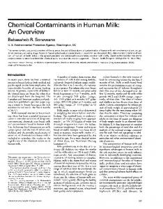
Fig. 3. Reweighing of the samples are shown. The new weight of sample si in proportion to the observation density is πi .
which is known as observation density is to be a Gaussian function G(µ, σ) where µ is the mean of the Gaussian and is located on the real measurement from the sensor and σ is its deviation. This distribution shows that the probability that the measurement be at the exact real position of the object has the highest value. Fig. 3 shows the reweighing of each sample according to the Gaussian function. It should be noted again that we have shown the observation density for a onedimensional case. A higher degree function needed for higher dimensional state spaces. This set of samples with their new probabilities forms the distribution that we were looking for i.e. p(xt |z1 , ..., zt−1 , zt )
890
Authorized licensed use limited to: Uppsala Universitetsbibliotek. Downloaded on January 8, 2010 at 03:13 from IEEE Xplore. Restrictions apply.
In the next time step t + 1, we use p(xt |z1 , ..., zt−1 , zt ) as the previous time distribution and we draw N new samples according to this distribution and we repeat the whole procedure. In the case of clutter where we have more than one measurement (in the case of this one dimensional example, if we have more than one point on the line and we want to track one of them), we reweigh each sample according to the nearest measurement. Since there is more than one sample in the process (in this case N samples), we need to pick one of them as the representative of the real position of the point at the current time step. There are different methods for performing this task. Choosing the sample with the highest weight (probability) or a sample whose weight is the median of the weights of the samples are two ways of selecting the representative sample. C. Tracking Mechanism for a Single Pan-Tilt-Zoom Camera Now we describe tracking an object with an uncalibrated camera which has the capability to pan and tilt to track the object while it can focus on the object with variable degrees of zoom. We define the state vector as the spherical coordinates of one specific point on the object of the interest. This point can be the center of mass of the object which is approximately determined by simple processing of the projected image of the object onto � the 2D image plane. �So the state vector is defined as: xt = θ θ˙ φ φ˙ r r˙ where θ and φ are angular ˙ φ˙ and r˙ are the components and r is the distance factor, θ, rate of change of these parameters respectively. The reason that we use spherical coordinates is that since the camera is uncalibrated and we know the angle of pan and tilt of the camera from its control section, it is more convenient and accurate to use this coordinate system rather than Cartesian coordinate system. Let us define the coordinate frame C in which we define the coordinate of the samples like what is shown in Fig. 4. The origin of this frame is located at the center of projection of the camera at an initial state and its z axis is perpendicular to the plane that the camera resides on and the y axis is perpendicular to the center of the image plane at an initial position of the camera. We choose N samples according to the probability distribution from the last time step p(xt−1 |z1 , ..., zt−1 ). Then we apply the dynamic model which we have assumed to be a linear first order equation to get a new set of samples. After that we reweigh each sample according to the observation from the camera. Having applied the dynamic model, we measure the real position of the object by using the camera. The measurement� � vector at time t has the form zt = θ θ˙ φ φ˙ r r˙ So we need to map the image plane data to the real spherical coordinates. At each time step the pan and tilt degree of the camera (θc and φc ) are known from the control hardware. To compute the spherical coordinates of the center of visible part of the object that is being tracked we should consider the deviation of that point from the current degree of pan and tilt (θc and φc ) considering the current zoom value (Fig. 4b). θI and φI ,
Fig. 4. (a) The setup for tracking a moving toy car on a table is shown. It is assumed that the image plane at all degrees of pan and tilt of the camera is a sphere which is shown in the schematic. Each sample has a projection on the image plane and we assume a depth for the samples. For example the ith sample si has the depth of ri . (b) A focused section of the image plane is shown. l1 and l2 are the projection of the optical axis of the camera in the current degree of pan and tilt (The solid red line) on the x-y and y-z plane respectively. θc is the angle between l1 and the x axis and φc is the angle between l2 and the z axis. O is the projection of one point of the object on the image plane.
the angular deviation of the object of interest from the center of image are evaluated using simple pinhole camera model. So θ and φ are defined as θ = θc − θI and φ = φc − φI . Now we should find the depth of the object (the r parameter in the measurement vector). By using the priori knowledge about the dimension of the object and the width and height of the object in the image plane, we can have an estimation that how far the object is from the center of projection of the camera. To compute the velocity components in the measurement vector at the current time step, we calculate the difference between the value of the other components of the measurement vector in the current and the last time step. After the measurement is done we reweigh each sample proportional to the observation density p(zt |xt ) which is assumed to be a six dimensional Gaussian whose mean is located on the nearest measurement to each sample by following the procedure which was described in the last subsection. Now we should pick one of the samples as the representative sample so that the agent changes its direction toward that sample. The sample that has the median of the weights of the samples is chosen as the estimated position of the object. Since the camera has a position control, we send to the camera the difference between the current direction of the camera and the direction of the chosen sample. Also the camera adjusts its focus according to the estimated distance of the object. Then we propagate the new probability distribution over the state space to next time step to continue tracking.
891
Authorized licensed use limited to: Uppsala Universitetsbibliotek. Downloaded on January 8, 2010 at 03:13 from IEEE Xplore. Restrictions apply.
III. MULTIPLE CAMERA TRACKING In this section, we describe the tracking algorithm using multiple pan-tilt-zoom cameras. Since there is a possibility of failure or occlusion of one camera, we increase the robustness of the system by increasing the number of cameras that track the object. Also different views of an object help us in reconstructing of its 3D structure. So we try to maximize the number of the cameras that track one object at each time step. It should be noted that each agent has as maximum zoom as possible on the object during the tracking. The amount of zoom depends on the dimensions of the projection of the seen object on the image plane. But extracting the object information (size, center of mass, etc.) in a zoomed view of an object is somehow unreliable and this unreliability is caused by this fact that there is a possibility that the object is not visible completely in the zoomed view. The non-visibility of parts of the object adds more noise in approximating the real position of the object. In this section we describe how we deal with this unreliability to increase the robustness of the probabilistic tracker. In the following subsections we explain the actions that each agent can take during the tracking. A. Cooperative Action Selection Each agent can take three actions during the tracking. These actions are: Zoom-out, Communication and Tracking. 1) Zoom-out: This action is taken by an agent when all of the agents have no idea about the position of the object. By taking this action each agent widens its field of view to cover more space and increase the probability of finding the object. 2) Communication: The other action that an agent can take is the communication action. This action is taken when at least one of the agents has an observation of the object. An architecture like the Blackboard architecture in [10] has been implemented for the coordination of the agents where a central unit applies the Condensation algorithm and uses the agents’ observation densities for finding a new probability distribution over the state space. The assumption is that the relative position of the cameras is known initially or will be determined through communication. Each agent has its own observation density which depends on the level of reliabilty of the agent. We denote this quantity by LRit which is the level of reliability of agent i at time t. As mentioned before, each agent has a level of reliabilty. This level of reliability determines how much the central unit can rely on the data of an agent. An agent has the highest level of reliability if it can observe the object completely. The other agents that see the object partially have a lower level of reliability. If two agents see an object partially, the agent that has less zoom value has higher level of reliability which means the data from a less focused camera is more reliable. We describe the algorithm for cooperative tracking of two agents but it is easily extendable to multiple agents. We assume a single general probability distribution over the state space (space of tracking) for all of the agents. As mentioned in the explanation of the Condensation algorithm
Fig. 5. Reweighing of each sample according to different agent’s observation density is shown. pi (zt |xt ) and pj (zt |xt ) are observation densities of agent i and agent j respectively. LRit > LRjt so the pj (zt |xt ) has a larger deviation.
we choose N samples proportional to the probability distribution from the previous time step i.e. p(xt−1 |z1 , ..., zt−1 ). After applying the dynamic model which is assumed to be a linear first order differential equation because of the mechanical limitation of the camera, we need to reweigh each sample according to the observation densities. At this step, each agent transmits its level of reliability and the measurement vector (which are the result of processing of the image plane data) to the central unit. We assume that the observation density for each agent is a Gaussian that changes over time. The central unit transforms the coordinates of the measurement vector to a reference world coordinate frame and uses the new measurement vector to find µ (the mean) of the Gaussian and uses level of reliability to determine the deviation (σ) of that. The deviation of the Gaussian for agent i at time t is proportional to inverse of the LRit which means that the observation density from an agent with higher level of reliability has less deviation and peak of the Gaussian is sharper. Like what is mentioned in the background section we reweigh each sample according to these observation densities and each sample is reweighed by the distribution whose mean is the nearest to that sample. Fig. 5 shows the reweighing of the samples considering that LRit > LRjt . A simple one dimensional case is shown in the following figure. After the central unit completed the reweighing of the samples, it broadcasts the sample with the median of weight of the samples to all of the agents as the current belief of the system for object position. The new probability distribution is normalized and propagated to the next time step as it is needed for tracking in the next time steps. 3) Tracking: After applying the Condensation algorithm, the central unit estimates the position of the object and broadcasts this estimate to all of the agents. Each agent adjusts its degree of pan and tilt according to the new estimate. The zoom value of each agent is determined according to the estimated distance of the object from the center of projection of the camera. IV. CONCLUSION An overview of a probabilistic tracker (the Condensation algorithm) which is able to model non-linear and non-Gaussian motions was presented. Then we applied the tracking algorithm to track an object according to multiple degrees of
892
Authorized licensed use limited to: Uppsala Universitetsbibliotek. Downloaded on January 8, 2010 at 03:13 from IEEE Xplore. Restrictions apply.
Fig. 6. The experimental setup with two cameras is shown in the picture. The crosses are the measured position of the object by the cameras.
freedom of one pan-tilt-zoom camera and the idea was to track an object with maximum possible zoom on it. After that, for increasing the robustness of tracking we added more pan-tiltzoom camera agents to track the object. We defined a level of reliability for each agent and used that value for reweighing of the samples and finding a new probability distribution over state space. The major disadvantage of the mentioned algorithm is that we can never know the exact position of the object which may cause some imperfections in tracking. Also a better dynamic model can result in a better tracking result. The computational requirements of this method of tracking are somehow high so the tracking is done in near real time. The performance can be improved by some methods such as [11] in which they have improved the efficiency by the use of adaptive size of sample sets. It should be noted that each agent can track the object itself without communicating with the central unit in the case of failure of the central unit, etc. This tracking system has many applications such as surveillance systems in buildings and parkings, tracking athletes in the sport fields while we can get a zoomed view of them.
Fig. 7. Sampling from f1 (x). A set of N samples are drawn randomly with a probability proportional to f1 (x). So we see more samples under high probability areas.
Fig. 8. (a) f2 (x) is shown in this figure. (b) Each sample is reweighed by the above equation. πj s are the new weights.
A PPENDIX A: FACTORED S AMPLING M ETHOD Suppose we have a probability distribution that is the result of multiplication of two other distributions. The factored sampling method is used to find an approximation to the probability density function by using samples from those two distributions. Assume f (x) = f2 (x)f1 (x), where f1 (x) and f2 (x) are two probability distributions. A set of samples s = {s1 , s2 , ..., sN } is drawn randomly from f1 (x) (Fig. 7). Then we find the probability assigned to each sample in proportion to f2 (x). The probability πj of the j th sample in proportion to distribution of f2 (x) is computed as follows: f2 (sj ) πj = �N , 1 f2 (sj )
j = 1, ..., N
(4)
So we have found a new sample set, where the distribution of the probabilities of the new samples tends to that of f (x), as N → ∞. Therefore, the distribution of the probability of these new samples is an approximation to the distribution f (x).
R EFERENCES [1] M. Isard and A. Blake. Condensation - conditional density propagation for visual tracking. International Journal on Computer Vision, 29(1):5– 28, 1998. [2] Q. Li and S. Payandeh. Multi-agent cooperative manipulation with uncertainty: A neural-net-based game theoretic approach. In IEEE International Conference on Robotics and Automation, pages 3607– 3612, Taiwan, 2003. [3] R. Grabowski, L. E. Navarro-Serment, C. J. J. Paredis, P. K. Khosla. Heterogeneous teams of modular robots for mapping and exploration. Autonomous Robots, 3(8):293–308, 2000. [4] W. Burgard, M. Moors, D. Fox, R. Simmons, S. Thrun. Collaborative multi-robot exploration. In Proceedings of IEEE International Conference on Robotics and Automation, pages 476–481, San Francisco, April 2000. [5] S. Kang, J. Paik, A. Koschan, B. Abidi, M. A. Abidi. Real-time video tracking using ptz cameras. In Proc. of SPIE 6th International Conference on Quality Control by Artificial Vision, pages 103–111, Gatlinburg, TN, May 2003. [6] B. Jung and G. S. Sukhatme. Detecting moving objects using a single camera on a mobile robot in an outdoor environment. In 8th conference on Intelligent Autonomous Systems, pages 980–987, Amsterdam, The Netherlands, March 2004. [7] R. Collins, O. Amidi, T. Kanade. An active camera system for acquiring multi-view video. In International Conference on Image Processing, Rochester, NY, September 2002. [8] S. Lim, A. Elgammal, L. S. Davis. Image-based pan-tilt camera control in a multi-camera surveillance environment. In IEEE ICME 2003, Special Session on Visual Surveillance, Baltimore, Maryland, July.
893
Authorized licensed use limited to: Uppsala Universitetsbibliotek. Downloaded on January 8, 2010 at 03:13 from IEEE Xplore. Restrictions apply.
[9] A. Makarenko and H. Durrant-Whyte. Decentralized Data Fusion and Control in Active Sensor Networks. In the 7th International Conference on Information Fusion (Fusion’04), pages 479–486 ,Stockholm, Sweden, 2004. [10] A. Ordean and S. Payandeh. Design and analysis of an enhanced opportunistic system for grasping through evolution. In Proceedings of the Third Conference on Advanced Robotics, Intelligent Automation and Active Systems, pages 453–459, 1997. [11] C. Kwok, D. Fox, M. Meila. Adaptive real-time particle filters for robot localization. In IEEE International Conference on Robotics and Automation 2003, pages 2836–2841, Taiwan, September 2003.
894
Authorized licensed use limited to: Uppsala Universitetsbibliotek. Downloaded on January 8, 2010 at 03:13 from IEEE Xplore. Restrictions apply.