AbstractâThe probabilistic multi-hypothesis tracker (PMHT) is an effective multiple target tracking (MTT) method based on the expectation maximization (EM) ...
IEEE TRANSACTIONS ON SIGNAL PROCESSING, VOL. 59, NO. 12, DECEMBER 2011
5721
Improved Probabilistic Multi-Hypothesis Tracker for Multiple Target Tracking With Switching Attribute States Teng Long, Member, IEEE, Le Zheng, Xinliang Chen, Yang Li, and Tao Zeng Abstract—The probabilistic multi-hypothesis tracker (PMHT) is an effective multiple target tracking (MTT) method based on the expectation maximization (EM) algorithm. The PMHT only uses the kinematic information to solve the problem of measurement to target association. However, in some applications, other information such as attribute measurements of targets may be available, which has potential to reduce misassociations and improve the tracking performance. Integrating attributes into the PMHT may suffer from the switch of attribute states and the instability of attribute measurements. In this paper, an attribute-aided association structure for the PMHT is proposed to consider the uncertainty in both attribute states and attribute measurements. The attribute characteristics are described by the hidden Markov model (HMM), and the joint probabilistic model of kinematic and attribute properties is derived. The attribute states are estimated by the Viterbi algorithm and the data association is improved by the extracted attribute information. Simulation results show that the proposed algorithm has better performance when the attributes of targets are available. Index Terms—Attribute, hidden Markov model, probabilistic multi-hypothesis tracker, Viterbi algorithm.
I. INTRODUCTION
O
NE of the major problems in multiple target tracking (MTT) is the association of tracks and measurements. “Hard association” algorithms such as the multi-hypothesis tracker (MHT) [1], [2] need to exhaustively list possible assignments, and suffer from an exponential growth of computational expense with time and the number of targets. The probabilistic multi-hypothesis tracker (PMHT) proposed by Streit [3], [4] avoids these problems. The whole time interval of PMHT is divided into batches, and the estimation of targets’ kinematic states is obtained by using the expectation-maximization (EM) algorithm [5] within each batch. The computation complexity of the PMHT grows linearly with the number of targets and the length of each batch. At present, improvements of the PMHT include nonlinear models [6], [7], target-maneuver [8], [9], and spread targets [10], [11]. In some applications, more information of the targets is provided to reduce the misassociations and improve the tracking Manuscript received January 21, 2011; revised June 10, 2011 and August 10, 2011; accepted August 17, 2011. Date of publication September 12, 2011; date of current version November 16, 2011. The associate editor coordinating the review of this manuscript and approving it for publication was Dr. Ta-Hsin Li. This work was supported by the National Natural Sciences Foundation of China (Grants 60890073 and 61001191). The authors are with the School of Information and Electronics, Beijing Institute of Technology, Beijing 100081, China (e-mail: chenxinliang123@126. com). Color versions of one or more of the figures in this paper are available online at http://ieeexplore.ieee.org. Digital Object Identifier 10.1109/TSP.2011.2167616
performance. Previous studies have been made to incorporate continuous features such as the size and intensity of the targets into the PMHT [12]–[14]. But the use of attributes is different. The attribute is defined as discrete sampling for target characteristics [15]–[17], such as the scatterer number and the type of radar used by target. As a result, attribute-aided association methods need to be studied. Davey did some research in the field and he proposed the PMHT-C method [18], [19]. The PMHT-C introduces a time-invariant confusion matrix to describe the relation between noisy attribute measurements and targets, and modifies the assignment weights accordingly. In the situations that only the instability of attribute measurements exists, the performance of the PMHT-C is superior to that of the original PMHT algorithm. The PMHT-C also has some limits. It assumes the confusion matrix to be constant in each batch, which indicates that the attribute states of targets would not switch. However, both the instability of the attribute observing process and the switch of attribute states exist in practice. A physical example is the scatterer number of high resolution radar targets. Influenced by false alarms and missed detections, observed scatterer number of a target fluctuates according to the probabilistic distribution determined by the attitude of the target. If the attitude of the target changes, the mismatch of the confusion matrix may occur to the PMHT-C and the tracking performance will decrease a lot. In this paper, the restrictive assumption in the PMHT-C is relaxed and an attribute-aided association framework for the PMHT is provided. The key to our proposed algorithm is the probabilistic integration of kinematic properties and attribute properties. S. Davey’s later work [19], [20] provides some illuming ideas. Dynamic state variables are used to represent targets’ prior probabilities and improve the tracking performance in cluttered environment. The same strategy is adopted and the relation of attribute states and attribute measurements is described by the hidden Markov model (HMM) when random variables are used to represent attribute states. On this basis, we obtain the posterior probability for the entire target states rather than only for the kinematic states. The expression for estimating the attribute states of targets is then derived. The extracted attribute information can be used to refined the assignment weights and improve data association. The structure of this paper is as follows: Section II introduces the mathematical model of the problem, reviewing the joint model of kinematic properties and attribute properties. In Section III the improved PMHT algorithm is introduced and some of its properties are discussed in Section IV. Simulation results are presented in Section V, and the factors that influence the performance of the proposed algorithm are analyzed. Conclusions are given in Section VI.
1053-587X/$26.00 © 2011 IEEE
5722
IEEE TRANSACTIONS ON SIGNAL PROCESSING, VOL. 59, NO. 12, DECEMBER 2011
II. PROBLEM FORMULATION A. Kinematic Characteristic targets, the In the tracking scenario, there are moves according to the discrete-time linear model
th one (1)
for . Here, the superscript is used to indicate that is the kinematic state of the th target. represents the state matrix and is an uncorrelated zero mean Gaussian noise with covariance . The kinematic states of all targets at time are defined as , and the states in the batch are . is defined as the index of the target that If the variable , then the generates the th observation at time , observation model is (2) In the above formula, the observation matrix is known. Prior probability of is defined as . The covariance of the true measurement from the th target is defined as , describing from (2), whereby in some cases variable is used to represent the covariance of measurement which is based upon the location of the observation [21]. In order to make the model more general, the measurement noise is rewritten as and variable is used to represent the covariance of measurement . Therefore, assuming clutter to be target , we have
(3) In (3), represents the probability distribution function (PDF) of the clutter, which is assumed to be continuous as a function of . Although unnecessary, is assumed to be uniform in most cases. Kinematic observations at time and in the whole batch are separately denoted as and where is the number of observations at time . Similarly, the assignment sets are defined as and .
Fig. 1. The joint model of kinematic and attribute properties.
Suppose the probability of attribute state switch does not vary with time, then is regarded as a constant, and could be . Therefore, the attribute state transirewritten as tion matrix of the th target is written as . 2) Attribute Measurement: If is the th attribute measurement at time , then we have the measurement sets and . If target generates the th measurement, that is, , then the conditional probability of the attribute measurement can be written as or . Assuming that the attribute measurements of different targets obey a known time-invariant probability distribution, we have (5) for the th target. Similarly, the observation matrix can be de. fined as Specifically, for measurements generated by clutter, the attribute observing process is much more stable than that of the targets. So it is convenient to define the observing probability for clutter as .
B. Attribute Characteristic The fluctuations of targets’ attribute measurements are caused by two factors. One is that different attribute measurements may be generated by a target in certain attribute model, the other is that the attribute model of a target may switch. In this paper, a state variable is introduced to characterize the attribute model of targets and the HMM is introduced to cope with both the switch of attribute states and the instability of attribute measurements. The mathematical description is as follows: 1) Attribute State: The switching process of attribute state is characterized by a first-order Markov model. Let be the attribute state of target at time , then we have . Let be the conditional probability that a switch of attribute state from to occurs at time , then we have (4)
C. Joint Model of Kinematic and Attribute Properties We have defined the kinematic states, kinematic measurements, attribute states and attribute measurements as above. Here their relation will be analyzed and the joint probabilistic distribution function of the state transition process and observation process will be derived. The relation of the , and can be described by a directed graphic model, as is shown in Fig. 1. Since no cycle exists, the assignments partition the graph into two parts: an upper subgraph for the kinematic properties and a lower subgraph for the attribute properties. According to [22] and [23], the kinematic properties and attribute properties are independent once is known. Applying the independence of kinematic and attribute properties, the joint probabilistic distribution function of the state transition process and
LONG et al.: IMPROVED PMHT FOR MULTIPLE TARGET TRACKING WITH SWITCHING ATTRIBUTE STATES
5723
observation process can be formulated via
(6)
(7) In the above formulas, the conditional probabilistic distriand are the sepabution rate simplified forms of and . In the original PMHT, the calculation of the assignment weights to complete the EM iteration only considers the kinematic properties. However, the assignment weights can be computed considering both kinematic and attribute information in this paper. The switch of attribute states is also taken into consideration. As a result, better data association performance will be obtained. III. IMPROVED PMHT ALGORITHM In Section II, the state set , observation set and assignment set are defined. To integrate attributes into the PMHT structure, an auxiliary function which is the expectation of the log-likelihood with respect to the missing assignments is built in this section. The maximum a posteriori (MAP) estimation of the kinematic states, attribute states are obtained through maximizing this auxiliary function.
(9) is the prior probability of . The where formal derivation of the prior probabilities is first done in [24] when the prior works made them parameters to be estimated by the EM algorithm [5]. Suppose all the targets have the same probability of detection , the prior probability of the targets is
(10) The number of clutter points is Poisson distributed with mean where represents the mean amount of clutter per unit volume and is the volume of the viewing area. Parameters and suggest the prior probabilities are influenced by the number of measurements and the number of targets. To calculate the expected log-likelihood function, the other of which we need . This can be element is obtained by the summation of (9).
A. Expected Log-Likelihood Function The derivation of the PMHT with switching attribute states is based on the HMM built in Section II. The auxiliary function in the th iteration is defined as
(8) According to the independence of the random variables suggested by (6) and (7), we have (11) Then, the is computed through the Bayesian formula [see (12) at the bottom of the page]. In the above formula, the weight is the probability conditioned on the event that the th measurement arises from target at time , the superscript of which amplifies the fact that the weight is computed from the th iteration. To make the notation correct if no measurement exists at certain time, the definition (13)
(12)
5724
IEEE TRANSACTIONS ON SIGNAL PROCESSING, VOL. 59, NO. 12, DECEMBER 2011
shall be included when for completeness [24]. The posterior association probability here relates to not only the kinematic states and the kinematic measurements, but also the attribute states and the attribute measurements. In the case that the estimation of attribute states is accurate, more measurements will be given the correct weights and the performance of data association will be better. Substituting (9) and (12) into (8) and neglecting all clutter terms [24], we have
where
(16) (17) should be added. The form of the synthetic observations in (16) and (17) are first given in [21], allowing each measurement to have a different covariance. The previous research assumed that all measurements have the same covariance [25]. In such cases, (16) and (17) can be simplified as
(18)
(19)
Applying the relation , and omitting the irrelevant components, the equivalent form of the expected log-likelihood function in the th iteration is
(14) and in (14) should be separately maxThen, can be perimized in the EM iteration. Maximizing formed indirectly by maximizing an equation with the same gradient. Omitting uncorrelated terms, the derivation can be transformed as
(20) In order to guarantee a smooth iteration, and are separately optimized in the M-step. The kinematic states is estimated by the Kalman smoother [26], running a backward smoothing operation on the track estimation resulting from the Kalman filter step. B. Estimation of the Attribute States (15)
Estimating the attribute states is discussed in this section. The auxiliary function of attributes in the th iteration can be
LONG et al.: IMPROVED PMHT FOR MULTIPLE TARGET TRACKING WITH SWITCHING ATTRIBUTE STATES
rewritten as
5725
2) Iteratively compute the node cost at each time and record the best path:
(24)
(25) (21) For simplicity, it is assumed that the attribute state transiand attribute observation probability tion probability are known, and the targets switch between possible attribute models. As can be seen in (21), can be decomposed independent determined by the index . as Therefore, maximizing the attribute auxiliary function can be achieved respectively for each by optimizing . For target , maximizing is equivalent to determining the best state sequence in batch . We have time steps and possible states for each time step. Each attribute state at will have a partial probability and a partial best path. The overall best path is achieved by choosing the state and choosing its partial best with the maximum path. The Viterbi algorithm, which was first presented in Andy’s famous 1967 paper [27], can be used to maximize here. The Viterbi algorithm only retains the best state sequence which leads to each possible attribute state at every time step [28]. Each state is regarded as a node in the dynamic model. is the node cost of the attribute state , then Suppose the maximum of all the sequences ending at state is , i.e.,
3) Terminate the iteration and determine the most likely final attribute state by finding the node with the highest : (26) (27) 4) Extract the attribute state sequence, following the path backwards from to : (28) The modified assignment weights are obtained by substituting the solution of the attribute state sequence into (12). The introduction of attributes may reduce the ambiguity in data association and correct the bias of tracking. In Section II, it is assumed for simplicity that the transition probability and observation probability of attribute states do not vary with time. However, the assumptions seem to be unnecessary here. If the variable in (24) and (25) is substituted by , and substituted by , the cases with time-varying attribute probability can be taken into consideration. Moreover, the constraint that the attribute observing model of clutter is time-invariant may also be relaxed. By introducing an “imaginary attribute state” of clutter, we are able to adjust the attribute observation model of clutter according to time and modify corresponding assignment weights to improve the data association. C. Iteration Initialization
(22) Thus, ending at state is maximized by selecting the best . The algorithm operates until the last time step . The best attribute state estimation for the batch is chosen from the best state sequences ending at each final attribute state. The whole process is conducted in four steps. 1) Initialize the node cost at a;
(23)
The PMHT requires an initial estimate for all of the states in the batch. As the algorithm is generally useless without a decent initial estimation [29], methods for state initialization are discussed here. For the initialization of kinematic states, methods have been detailedly discussed in [21], [24], [30], and [31]. The batch can either slide one step [31] or multiple steps forward [21], different initialization methods may be used. This paper mainly contributes for integrating the attributes into the PMHT. Thus, the initialization methods for kinematic states show no difference. All aforementioned batch sliding strategies and initialization methods can be directly used without any modification. Initializing the attribute states is different from initializing the kinematic states because the variables are discrete. In this paper, the attribute states in the overlap area of the new batch are initialized by the state estimation of the previous batch. As some initialized states is smoothed by the future observations, “information incest” is introduced. To initialize the attribute states which are out of the overlap area, the attribute prediction is needed.
5726
IEEE TRANSACTIONS ON SIGNAL PROCESSING, VOL. 59, NO. 12, DECEMBER 2011
Fig. 2. The initialization of attribute states.
A simple way is to use the attribute state of the last node in the overlap area. Although the switch of the attribute states may happen, the initialization error will be revised in the process of the EM iteration and the use of attributes will provide benefits to the data association. For example, for the multi-shift batches in Fig. 2, the attribute states at time 5, 6 are initialized by the attribute state at time 4. However, the attribute initialization method mentioned above does not work well in some specific situations. If an element , i.e., the observation probability centralizes on state , the algorithm will put too much confidence in the attribute prediction. Then, a switch of attribute state may cause measurements from the wrong target to be assigned to a track and the state error will become larger when the targets move farther. Thus, the initialization method should be adjusted according to the attribute observation probability. A “delayed initialization” strategy is used when the observation probability centralizes on certain state. The assignment weights are first computed by only using the kinematic measurements. Suppose is the most left time node out of the overlap area, then the attribute states for target are initialized by optimizing
(29) This initialization method relies on the kinematic predictions and kinematic observations, so more “information incest” is introduced, which may lead to the local convergence of the EM iteration. In the cases that the attribute observation probability does not centralize on certain state, initializing the attribute states using the last node of the overlap area is preferred. Otherwise, the initialization of attribute states using (29) is better. D. The Algorithm The derivation of the improved PMHT with switching attribute states (PMHT-SA) has been given. The whole process of the proposed algorithm is similar to that of the original PMHT [25]. The difference is that the proposed algorithm needs to estimate the attribute state sequence of the targets. The algorithm can be summarized as follows. 1) Set the initial state estimate and for the targets.
that the th mea2) Calculate the assignment weight surement is generated by target at time . 3) Refine the measurements and covariance by using the weights . 4) Run the Kalman smoother and solve the kinematic states , by using the modified measurements with covariance . The initial state and corresponding state covariance should not be smoothed. 5) Estimate the attribute states by using the Viterbi algorithm. con6) Repeat steps 2–6, until the function verges. 7) Slide the batch window forward and go to 1. The iteration is supposed to stop when the expected log-likelihood function converges. As the convergence of the PMHT is guaranteed [3], the number of iterations can also be fixed in some applications. IV. SPECIAL CASES The proposed algorithm can be regarded as an logical extension of the original PMHT algorithm. State variables have been introduced to characterize the attribute model of the targets. Three special cases of attribute states and corresponding performance of the proposed algorithm are analyzed in this section. A. Absence of Attribute State Switch In the case that the attribute states of the targets don’t change, only the instability of attribute measurements exists. Two completely different cases may happen characterized by the initial attribute states in this situation. Suppose no false alarms or missed detections exist and the attribute observation matrix for different targets are the same. If the attribute states of the targets are the same, the weights in the th iteration will become (30)
Equation (30) is the same as the assignment weight of the original PMHT algorithm [25], that is, the attribute cannot provide any assistance to the tracking. In the other case, the initial attribute states of the targets are different. Then the observing processes of the targets are different in every time step of the batch. At this time, the assignment weights become (31)
The structure of here is exactly the same as that of the PMHT-C [18]. Thus, the proposed algorithm is simplified to the PMHT-C in the case. B. Uniformly Random Attribute State Switch If the model switch of attributes is uniformly random, then we have , where is the number of the possible attribute states. Omitting constant terms, the auxiliary function
LONG et al.: IMPROVED PMHT FOR MULTIPLE TARGET TRACKING WITH SWITCHING ATTRIBUTE STATES
of the attribute states can be rewritten as
(32) The proposed algorithm estimates the attribute states by using the prior knowledge of both the temporary correlation of attribute states and the distribution of attribute observations. In is irrelevant to the attribute transition proba(32), bility, meaning that it is impossible to make use of the temporary correlation of attribute states. Therefore, the estimated attribute states at time is determined by the observation that has the maximum assignment weight and the usage of attributes provides no benefit to the EM convergence as a result. C. Attribute State Overlap Apart from the attribute state transition probability, the overlap of attribute states is another important factor that influences the improvement brought by the attributes. When different targets have the same type of attribute measurements or attribute states, the attribute information can not provide any assistance to the data association. The attribute characteristic combinations that invalidate the attribute-aided association are defined as the attribute overlap in this paper. For multiple targets tracking with attributes, four types of attribute property combinations for different targets exist: 1) attribute states and attribute measurements are the same; 2) attribute states are the same but attribute measurements are different; 3) attribute measurements are the same but attribute states are different; 4) attribute states and attribute measurements are different. In Case 1 and Case 2, the overlap of attribute states occurs. In Case 3, only the overlap of attribute measurements exists. The model of the PMHT-C only includes the attribute overlap of the observing process, which is shown in Case 3. However, the attribute state overlap in Case 1 and Case 2 cannot be neglected in this paper. The general form of the assignment weights when the attribute state overlap happens is derived here as (33), shown at the bottom of the page. When the overlap of attribute states happens, the use of the attributes only contributes for distinguishing targets and clutters. However, it does not help to separate different targets. At this time, little improvement is made for the multiple target tracking. A simple example is used to illustrate the influence of the attribute state overlap. Consider one scan with two targets, where the targets’ kinematic state estimations from the previous EM iteration are and with variance of ob. For a certain measurement, the assignment servation
5727
weight for track 1 is defined as , and the weight for track 2 is defined as . As is discussed in [19], for the original PMHT, the assignment weight of a measurement is simply determined by its position. When the attribute measurement is unavailable, the crossover point of the weight curves is the geometric midpoint of the two tracks. Track 1 will be preferred over track 2 if the measurement is closer to it and visa versa. If the attribute measurement is available, the weight functions will depend on the true source of the measurement and better tracking performance will be obtained. Assuming two types of attribute states and attribute measurements exist, the attribute observation probability is and for 1, 2. For clutter, and . In Fig. 3(a), the weight curves we have of the measurement when the attribute state estimations from the previous EM iteration are . Fig. 3(b) shows the weight curves of the measurement in the case that the attribute state estimations from the previous iteration are and . Thus, the overlap of attribute states exists in Fig. 3(a) and no overlap of attribute states exists in Fig. 3(b). As can be seen from the figure, there are different weight characteristics depending on the attribute states. When no overlap of attribute states exists, the weight curves extend from the track before dropping down and the crossover points of and are far away from the geometric midpoint of the two tracks. However, in the cases that the overlap of attribute states exists, the shift of the curves is much less and the crossover points are close to the geometric midpoint of the tracks, indicating that less improvement can be made for the data association. As is analyzed in (33), the attribute measurement here contributes nothing to discriminating from the two targets. V. SIMULATION RESULTS A. Model and Parameter Values The kinematic model in simulation is two-dimensional; that is, with reference to (1) and (2), we have
(33)
5728
IEEE TRANSACTIONS ON SIGNAL PROCESSING, VOL. 59, NO. 12, DECEMBER 2011
Fig. 3. The assignment weight curves (a) when the overlap of attribute states exists and (b) when the overlap of attribute states does not exist.
for , with snapshots of measurements . The targets move according to and sampling interval a piecewise constant white acceleration model [32]. Measurements are presented to the processor as positions in and coordinates, where the observation covariance matrix is diagonal. Targets are detected with a probability of , and there are false alarms whose number is Poisson distributed according to clutter density at each scan, generated uniformly in a viewing rectangle bounded by . Some notes and parameters of the simulation are shown as follows. 1) In all the simulation scenarios, two targets exist, separately initialized by the kinematic and state . Thus, a cross may happen at about . 2) The measurements generated by different targets have the same standard deviation . 3) The PMHT algorithm is known as putting too much confidence in the prediction, thus may easily lose the tracks. So both the tracks moving in straight line and tracks moving non-straightly are used for the simulation, controlled by . A typical run of the first situation is shown in Fig. 4. We choose , and to generate an easier scenario for tracking. Fig. 5 shows a typical run for the second situation, we choose to form non-straight trajectories. The detection probability is set to be 0.9 and the clutter density is . Thus, the second tracking scenario is more challenging. 4) For the first simulation scenario, tracks seldom get lost. So the performance measure is the position root mean-squared
RMSE
error (RMSE), that is [see (34), shown at the bottom of the and , respectively, reppage]. In (34), resent the estimated position and true position of target at time and the subscript represents the th simulation. is the number of Monte Carlo simulations in which is the number of the targets for each no track is lost and simulation. 5) Since tracks may be easily lost in the second situation, the proportion of tracks not lost is used to evaluate the tracking performance. A track loss is declared if at any time step
(35) 6) Various probabilities of attribute transition and attribute observation are explored. In each of the simulation scenario, the targets switch between two attribute states. Two types of attribute measurements may be generated by an attribute state. We use the attribute state transition probabilities and attribute observation probabilities ; that is, there are 2 situations above, and each of them is explored for 18 subcases. 7) The attribute observing probability for clutter is set to be and . In all cases, simulations are run over 5000 random realizations. To avoid irrelevant track initiation issues, the PMHTs in the first batch are initialized by the correct initial state and projecting a constant velocity path from this point. The covariance . matrix is initialized as
(34)
LONG et al.: IMPROVED PMHT FOR MULTIPLE TARGET TRACKING WITH SWITCHING ATTRIBUTE STATES
5729
= 1 2 10
Fig. 4. A typical run of the first simulation scenario with � , P : and � . All the algorithms can maintain the tracks ,� successfully.
=1
=01
= 20
Fig. 6. Position RMSE and assignment weights as a function of time for the first situation. (a) Position RMSE [m]. (b) Assignment weight.
= 2 2 10
Fig. 5. A typical run of the second simulation scenario with � , P : ,� and � . The original PMHT and PMHT-C lose a track at the crossover point of the trajectories, while the improved PMHT maintains the tracks successfully.
= 09
=1
= 20
B. Tracking Performance The performance comparison of the original PMHT, the PMHT-C and the proposed algorithm is offered. The length of the sliding batches is 10, with a skip parameter of three time steps. It means that the window grows to a maximum of length 10. After the tenth time step, the window slides. For each batch, the PMHT is performed until the mean difference of position estimations between two iterations is less than 0.1. For batch initialization, the smoothed state estimation from the previous batch is regarded as the initial value of the new batch in the overlap area of the batches. The kinematic states for the rest of the batch are initialized by the Kalman prediction from the last time step in the overlap area. The covariance estimations produced by the Kalman smoother is set to be the new covariance when the window slides. For the proposed algorithm, the attribute states out of the overlap area between batches are initialized by the attribute state of the last node in the overlap area when . Otherwise, the attribute states are initialized through optimizing (29).
In Fig. 6(a), the mean square position errors are presented and as a function of time for the first situation with . At the beginning of the tracks, the estimate error is very low. This is due to the fact that the initialization uses the true value of the target state. When the two targets become close, the assignment weights of the targets deviate and the position RMSE of the targets becomes larger due to the increase of ambiguity in assignments. In the first situation where the targets move straightly, the proposed algorithm performs better than the original PMHT and the PMHT-C. Its overall performance gain over the original PMHT is 10.2% in a cross segment defined as . However, the PMHT-C is limited by the switch of attribute states, so its performance is even worse than the original PMHT. Apart from the RMSE in position, it is also of interest to study the average assignment weights of the trajectories over time. In Fig. 6(b), the -axis represents the average weight that the measurement generated by target 1 is assigned to the correct source. Integrated measurements are calculated through (18). Therefore, the greater is , the closer to the true value is the modified observation. As can be seen, the proposed alat is 19% higher gorithm’s assignment weight than that of the original PMHT, which means that more measurements are given with correct weights.
5730
IEEE TRANSACTIONS ON SIGNAL PROCESSING, VOL. 59, NO. 12, DECEMBER 2011
Fig. 7. The percentage of tracks not lost and the assignment weights as a function of time for the second situation. (a) Track-in percentage. (b) Assignment weight.
A bit unexpectedly, the weight curve of the PMHT-C is better than the original PMHT in the cross segment. It means that the attribute measurements can be used to distinguish the targets to some degree, and some benefits can be obtained in the cross segment. However, the improvement in assignment weights is limited by the switch of attribute states. So the assignment weights for example. become even worse in other segments, Thus, the overall position RMSE of the PMHT-C is higher than the original PMHT. Fig. 5 shows a typical run of the second situation. The original PMHT and PMHT-C lose a track at the crossover point of the trajectories, while the improved PMHT successfully maintains tracking by using the attributes. For comparison of the three algorithms, the track-in percentage at each time step is calculated. As the time goes by, the assignment weight in Fig. 7(b) decreases, showing more ambiguity in data association. Thus, the estimation bias becomes larger and more tracks are lost. The track-in performance of the three algorithms in the second simulation scenario is shown in Fig. 7(a), with and . Missed detections, false alarms and interference brought by multiple targets are the cause of the track losses. The result shows that the proposed algorithm is the best in track-in percentage when the tracks are not straight lines. The performance gain is 4.18% at the last time step over the original PMHT algorithm. So it is reasonable to conclude that the improved algorithm can relax PMHT’s problem by using the attributes. In order to compare the performance of the proposed algorithm with different attribute state transition probability and the attribute observation probability , a group of simulations are carried out with and . The performance gain brought by the attributes can be obtained by comparing the PMHT-SA and the original PMHT. It is noticeable that sometimes the proposed algorithm shows slight improvement over the original PMHT when . This is because the attribute observation probability of clutter is used to refine the assignment weights and thus reduces the interference of clutter observations. However, this improvement is usually small and can be neglected. Fig. 8(a) shows the simulation results in the first situation. as function of the The overall RMSE in segment
observation probability is given. The proposed algorithm is better than the original PMHT in all cases. When or increases, the correct rate of attribute state estimation decreases and the performance gain brought by the attributes is reduced. The proposed algorithm performs best at and . Little improvement can be seen when . In the second situation, the track-in percentage at the last time step is maximized at and , as is shown in Fig. 8(c). The higher is the attribute transition probability , the lower is the track-in percent. Likewise, when , the track-in percentage decreases with the decline in . Considering the two typical cases of simulation, we can conclude that 1) The performance gain brought by the attributes will decrease with the decline in . When , in (21) becomes insensitive to the estimation of the attribute state sequence, meaning that the correlation of attributes in time decreases and more confidence is put in the observations. Therefore, is easier to be influenced by the weights and to converge to local maximization. 2) When , the tracking performance is often reduced. The main reason of this experimental result is that and become insensitive to the atdue to the decline in . So the tribute measurement ability to correct the data association is reduced and the performance gain is limited. An exception of the second conclusion happens in Fig. 8(c) at . Compared with , the track-in percentage is lower, indicating that less improvement can be achieved by using the attributes. This is because the algorithm puts too much confidence in the attribute observation when the attribute observation probability concentrates on a certain state. If a mistake in attribute state estimation occurs, the assignment weight of the true source is set to be low and the mistake is hard to be corrected, and then the track may be lost as a result. This phenomenon seldom happens in the first situation. As the process noise is low, the estimate of kinematic states is accurate, which provides much help to the initialization of attribute states. Thus, the probability of mistaken attribute state initialization is relatively small and the performance of data association is improved. However, in a challenging situation where the targets
LONG et al.: IMPROVED PMHT FOR MULTIPLE TARGET TRACKING WITH SWITCHING ATTRIBUTE STATES
5731
Fig. 8. Tracking performance of the proposed algorithm for various attribute transition probability and attribute observation probability. (a) Overall position RMSE in the cross segment for the first situation. (b) Correct rate of attribute state estimation for the first situation. (c) Track-in percentage at the last time step for the second situation. (d) Correct rate of attribute state estimation for the second situation.
do not move straightly, the kinematic state estimation provides less help and more tracks will be lost. C. Analysis of the “Information Incest” According to Section III-C, the “information incest” is introduced in the process of attribute state initialization. So a simulation is carried out to see whether the improvement brought by the use of attributes is sensitive to the “information incest.” For each batch, a tradeoff exists between how far the batches slide and how much “information incest” is allowed. The attribute probabilities are set to be and . The batch skip parameter varies from 1 to 9, with a step of 1. In particular, the batches are single-shifted when the skip parameter is set to be 1 and there is no “information incest” when the skip parameter is set to be 9. The original PMHT, PMHT-C and PMHT-SA are run in the simulation. Fig. 9 and Fig. 10 shows the performance of the algorithms in both situations. In the first situation, the proposed algorithm performs best with single-shift batches. However, in the second situation, it performs best when the length of batch slide equals to 3. The performance gain of the proposed algorithm over the original PMHT can be seen from the figures. In the first situation, the variation of the performance gain never exceeds 0.1812 m. In the second situation, the variation of the improved track-in
Fig. 9. PMHTs’ mean position RMSE [m] in the cross segment (15 for the first situation (a typical run is shown in Fig. 4).
t
30)
percentage never exceeds 1.12%. As the variation of the performance gain is small, it can be concluded that the improvement brought by the attribute-aided association is insensitive to the “information incest.”
5732
IEEE TRANSACTIONS ON SIGNAL PROCESSING, VOL. 59, NO. 12, DECEMBER 2011
Fig. 10. PMHTs’ track-in percentage in the second situation (a typical run is shown in Fig. 5).
VI. CONCLUSION In this paper, an attribute-aided association framework for the PMHT is presented. In order to take both attribute state switching and attribute measurement fluctuation into consideration, the proposed algorithm models the attributes by using the HMM. Based on the probabilistic model, the attribute states of the targets are estimated by the Viterbi algorithm and the extracted attribute information is used to improve the performance of data association. Simulations are made for the original PMHT, the PMHT-C and the proposed PMHT-SA algorithms, with various skip parameters. The results demonstrate that the proposed algorithm has the best performance in all situations. It has also been shown that the proposed algorithm is insensitive to the “information incest” introduced in the process of attribute state initialization. Future work will focus on an application of the PMHT-SA to real radar data.
REFERENCES [1] S. Blackman, “Multiple hypothesis tracking for multiple target tracking,” IEEE Aerosp. Electron. Syst. Mag., vol. 19, no. 1, pp. 5–18, 2004. [2] S. Blackman and R. Popoli, Design and Analysis of Modern Tracking Systems. Noorwood, MA: Artech House, 1999, vol. 685. [3] R. Streit and T. Luginbuhl, “A probabilistic multi-hypothesis tracking algorithm without enumeration and pruning,” in Proc. 6th Joint Data Fusion Symp., 1993, pp. 1015–1024. [4] C. Rago, P. Willett, and R. Streit, “Direct data fusion using the PMHT,” in Proc. IEEE Amer. Autom. Control Conf., 1995, vol. 3, pp. 1698–1702. [5] A. Dempster, N. Laird, and D. Rubin, “Maximum likelihood from incomplete data via the EM algorithm,” J. Roy. Statist. Soc. B, Methodol., vol. 39, no. 1, pp. 1–38, 1977. [6] M. Efe, Y. Ruan, and P. Willett, “The pedestrian PMHT,” in Proc. IEEE 5th Int. Conf. Inf. Fusion, 2002, vol. 2, pp. 838–845. [7] E. Giannopoulos, R. Streit, and P. Swaszek, “Probabilistic multi-hypothesis tracking in a multi-sensor, multi-target environment,” in Proc. IEEE 1st Aust. Data Fusion Symp. (ADFS), 1996, pp. 184–189. [8] Y. Ruan, P. Willett, and R. Streit, “The PMHT for maneuvering targets,” in Proc. IEEE Amer. Control Conf., 1998, vol. 4, pp. 2432–2433. [9] Y. Ruan and P. Willett, “Multiple model PMHT and its application to the benchmark radar tracking problem,” IEEE Trans. Aerosp. Electron. Syst., vol. 40, no. 4, pp. 1337–1350, 2004. [10] T. Luginbuhl and P. Willett, “Estimating the parameters of general frequency modulated signals,” IEEE Trans. Signal Process., vol. 52, no. 1, pp. 117–131, 2004.
[11] R. Streit, “Tracking on intensity-modulated data streams,” Naval Undersea Warfare Center, Newport, RI, Tech. Rep. 11,221, 2000. [12] T. Luginbuhl and R. Streit, “Incorporating amplitude information into the PMHT using shot-noise models,” in IEE Colloquium on Target Tracking: Algorithms and Applications, 1999, p. 13-1, IET, Ref. No. 1999/090, 1999/215. [13] M. Wieneke and W. Koch, “Probabilistic tracking of multiple extended targets using random matrices,” in Proc. SPIE, 2010, vol. 7698, p. 769812. [14] P. Willett and S. Coraluppi, “MLPDA and MLPMHT applied to some MSTWG data,” in Proc. 9th Int. Conf. Inf. Fusion, Florence, Italy, 2006, vol. 10, pp. 1–8. [15] O. Drummond, “On categorical feature-aided target tracking,” in Proc. SPIE, 2003, vol. 5204, p. 544. [16] O. Drummond, “Integration of features and attributes into target tracking,” in Proc. SPIE, 2000, vol. 4048, p. 610. [17] P. Singer and A. Coursey, “Feature aided tracking (FAT),” in Proc. SPIE, 2004, vol. 5428, p. 249. [18] S. Davey, D. Gray, and R. Streit, “Tracking, association, and classification: A combined PMHT approach,” Digit. Signal Process., vol. 12, no. 2–3, pp. 372–382, 2002. [19] S. Davey, “Extensions to the probabilistic multi-hypothesis tracker for improved data association,” Ph.D. dissertation, School of Electrical and Electronic Eng., Univ. of Adelaide, Adelaide, South Australia, 2003. [20] S. Davey and D. Gray, “Integrated track maintenance for the PMHT via the hysteresis model,” IEEE Trans. Aerosp. Electron. Syst., vol. 43, no. 1, pp. 93–111, 2007. [21] M. Wieneke and W. Koch, “The PMHT: Solutions for some of its problems,” in Signal Data Process. Small Targets, 2007, vol. 6699, pp. 1–12. [22] J. Kim and J. Pearl, “A computational model for causal and diagnostic reasoning in inference systems,” in Proc. 8th Int. Joint Conf. Artif. Intell., 1983, pp. 190–193, Citeseer. [23] C. Bishop, Pattern Recognition and Machine Learning. New York: Springer, 2006, vol. 4. [24] D. F. Crouse, M. Guerriero, and P. Willett, “A critical look at the PMHT,” Adv. Inf. Fusion, vol. 4, pp. 93–116, 2009. [25] P. Willett, Y. Ruan, and R. Streit, “PMHT: Problems and some solutions,” IEEE Trans. Aerosp. Electron. Syst., vol. 38, no. 3, pp. 738–754, 2002. [26] M. Grewal and A. Andrews, Kalman Filtering: Theory and Practice. Englewood Cliffs, NJ: Prentice-Hall, 1993. [27] A. Viterbi, “Error bounds for convolutional codes and an asymptotically optimum decoding algorithm,” IEEE Trans. Inf. Theory, vol. 13, no. 2, pp. 260–269, 1967. [28] H. Lou, “Implementing the Viterbi algorithm,” IEEE Signal Process. Mag., vol. 12, no. 5, pp. 42–52, 1995. [29] Y. Ruan and P. Willett, “The turbo PMHT,” IEEE Trans. Aerosp. Electron. Syst., vol. 40, no. 4, pp. 1388–1398, 2004. [30] P. Willett, Y. Ruan, and R. Streit, “A variety of PMHTs,” in Proc. Workshop Probabilistic Methods in Multi-Target Tracking, ENST, Paris, France, 1998. [31] C. Rago, P. Willett, and R. Streit, “A modified PMHT,” in Proc. Conf. Inf. Sci. Syst., 1995, pp. 647–652. [32] Y. Bar-Shalom and X. Li, Estimation and Tracking-Principles, Techniques, and Software. Norwood, MA: Artech House, 1993.
Teng Long (M’99) received the B.S. degree in electronic engineering from the University of Science and Technology of China (USTC), Hefei, China, in 1989 and the M.S. and Ph.D. degrees in electrical engineering from the Beijing Institute of Technology (BIT), Beijing, China, in 1991 and 1995, respectively. From January 1999 to August 1999, he was a Visiting Associate Professor with the Department of Electrical Engineering, Stanford University, Stanford, CA. From March 2002 to September 2002, he was a Visiting Scholar with the Department of Electric Engineering, London University, London, U.K. Since September 2000, he has been a Full Professor with the Department of Electronic Engineering and the Director of the Institute of Radar Technology, Beijing Institute of Technology, Beijing, China. His research interests include radar system, array processing, and synthetic aperture radar.
LONG et al.: IMPROVED PMHT FOR MULTIPLE TARGET TRACKING WITH SWITCHING ATTRIBUTE STATES
5733
Le Zheng was born in the Province of Hebei, China, in 1987. He received the B.S. degree in communication engineering from Northwestern Polytechnical University (NWPU), Xi’an, China, in 2009. He is currently working towards the Ph.D. degree in electrical engineering at Beijing Institute of Technology (BIT), Beijing, China. His research interests lie in the areas of radar system, statistical signal processing, and data fusion.
Yang Li received the B.S. degree in 2002 and the Ph.D. degree in 2007, both from the Department of Electronic Engineering, Beijing Institute of Technology, China. He joined the teaching staff of the Beijing Institute of Technology in 2007. His research interests include digital signal processing and statistical signal processing, with applications to radar systems.
Xinliang Chen was born in Hubei Province in China. He received the Bachelor’s degree in electronic engineering from the Department of Physical Science and Technology, Wuhan University, China, in 2005 and the Ph.D. degree from Institute of Semiconductor, Chinese Academic of Science, in 2010. He is currently a Postdoctoral Research Fellow at the Department of Electronic Engineering, Beijing Institute of Technology, China. His research interests include statistical signal processing and machine learning, with applications to radar systems.
Tao Zeng received the Bachelor’s and Ph.D. degrees from the Department of Electronic engineering, Beijing Institute of Technology (BIT), Beijing, China, in 1994 and 1999, respectively. He joined the teaching staff of the BIT in 1999. His research interests include SAR imaging technology and real-time radar signal processing.